1、环境配置
1.1 jupyter notebook 可以做哪些事情？
1.2 使用清华源进行安装　tensorflow-gpu　版
首先创建虚拟环境，参照：conda创建、查看、删除虚拟环境
cuda安装和版本：
GPU support
https://blog.csdn.net/dudu/article/details/
安装好cudnn后

pip install pip -U pip config set global.index-url https://pypi.tuna.tsinghua.edu.cn/simple pip install tensorflow-gpu==2.0.0 -i https://pypi.tuna.tsinghua.edu.cn/simple 

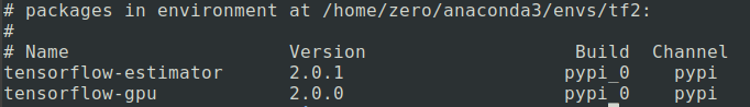
安装好后使用以下命令可查看安装的Tensorflow及版本号

讯享网conda list tensorflow 

讯享网
利用python行打印代码：

import tensorflow as tf print(tf.__version__) # 2.0.0 

2、数据操作
2.1　创健tensor

讯享网创建常量 x = tf.constant(range(12)) print(x.shape) 改变形状 # (12,) X = tf.reshape(x,(3,4)) 创建元素为１的向量 tf.ones((3,4)) 

按元素乘法：

X * Y #除了按元素计算外，我们还可以使用matmul函数做矩阵乘法。下面将X与Y的转置做矩阵乘法。由于X是3行4列的矩阵，Y转置为4行3列的矩阵，因此两个矩阵相乘得到3行3列的矩阵。 Y = tf.cast(Y, tf.int32) tf.matmul(X, tf.transpose(Y)) 

2.2向量的拼接

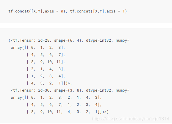
我们也可以将多个tensor连结（concatenate）。下面分别在行上（维度0，即形状中的最左边元素）和列上（维度1，即形状中左起第二个元素）连结两个矩阵。可以看到，输出的第一个tensor在维度0的长度（ 6 ）为两个输入矩阵在维度0的长度之和（ 3+3 ），而输出的第二个tensor在维度1的长度（ 8 ）为两个输入矩阵在维度1的长度之和（ 4+4 ）。

x.shape = (3, 4) 简单理解就是3句话,每句话4个字
y.shape = (3, 4)
concate axis=0，即沿 0 轴拼接，为 (3+3, 4)
concate axis=1，即沿 1 轴拼接，为 (3, 4+4)

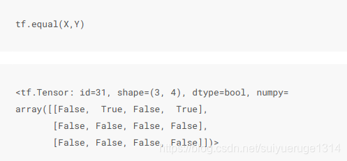
使用条件判断式可以得到元素为0或1的新的tensor。以X == Y为例，如果X和Y在相同位置的条件判断为真（值相等），那么新的tensor在相同位置的值为1；反之为0。

对tensor中的所有元素求和得到只有一个元素的tensor。

讯享网tf.reduce_sum(X) 

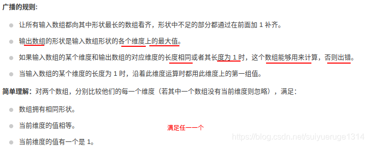
2.3　广播机制

前面我们看到如何对两个形状相同的tensor做按元素运算。当对两个形状不同的tensor按元素运算时，可能会触发广播（broadcasting）机制：先适当复制元素使这两个tensor形状相同后再按元素运算。

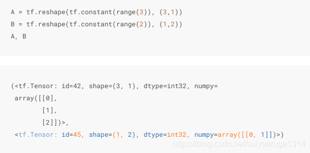
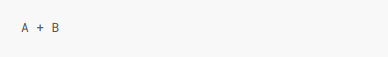
由于A和B分别是 3行1列 和 1行2列 的矩阵，如果要计算A + B，那么A中第一列的3个元素被广播（复制）到了第二列，而B中第一行的2个元素被广播（复制）到了第二行和第三行。如此，就可以对2个3行2列的矩阵按元素相加。

更细来说即： A(3,1) -> (3, 2)； B(1,2) -> (3, 2)，即前一个向量决定行后一个向量决定列，有点像矩阵乘法

Ａ 广播变换　-> [[0, 0], + B 广播变换　－> [[0, 1], [1, 1], [0, 1], [2, 2]] [0, 1],]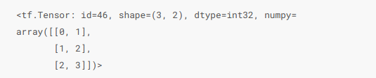 

这个例子比较简单，其实广播机制是一个更具体来说：参考: https://zhuanlan.zhihu.com/p/

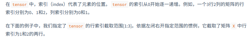
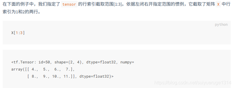
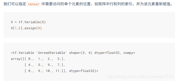
2.4 索引


tensor.assign() 重新赋值

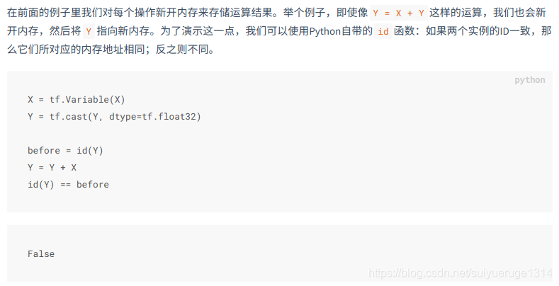
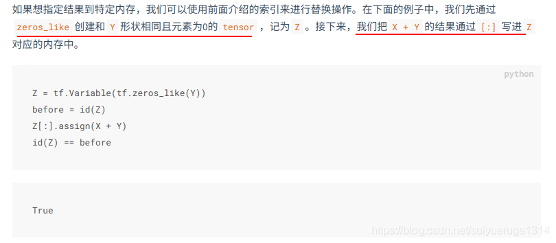
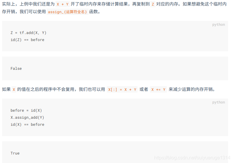
2.5 内存开销（assign_{运算符全名}）



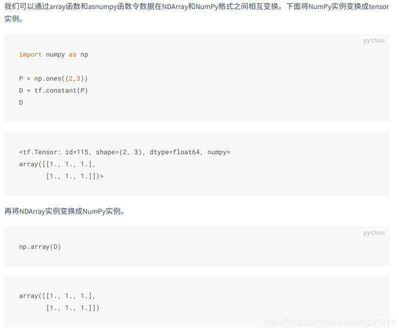
2.6 tensor 和 NumPy 相互变换

3、自动求梯度

在深度学习中，我们经常需要对函数求梯度（gradient）。本节将介绍如何使用tensorflow2.0提供的GradientTape来自动求梯度。

3.1 简单示例

讯享网创建变量ｘ，使用tf.Variable(), tf.constant()是创建常量 x = tf.reshape(tf.Variable(range(4), dtype=tf.float32),(4, 1)) 

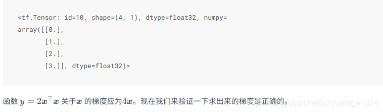
with tf.GradientTape() as t: t.watch(x) y = 2 * tf.matmul(tf.transpose(x), x) dy_dx= t.gradient(y, x) # 结果如下: <tf.Tensor: id=30, shape=(4, 1), dtype=float32, numpy= array([[ 0.], [ 4.], [ 8.], [12.]], dtype=float32)> 

3.2 多次调用

默认情况下，调用 GradientTape.gradient() 方法时， GradientTape 占用的资源会立即得到释放。通过创建一个持久的梯度带，参数 persistent=True, 可以计算同个函数的多个导数。这样在磁带对象被垃圾回收时，就可以多次调用 ‘gradient()’ 方法。例如：

讯享网with tf.GradientTape(persistent=True) as g: g.watch(x) y = x * x z = y * Y dz_dx = g.gradient(z, x) # 108.0 (4*x^3 at x = 3) dy_dx = g.gradient(y, x) # 6.0 dz_dx,dy_dx  WARNING:tensorflow:Calling GradientTape.gradient on a persistent tape inside its context is significantly less efficient than calling it outside the context (it causes the gradient ops to be recorded on the tape, leading to increased CPU and memory usage). Only call GradientTape.gradient inside the context if you actually want to trace the gradient in order to compute higher order derivatives. WARNING:tensorflow:Calling GradientTape.gradient on a persistent tape inside its context is significantly less efficient than calling it outside the context (it causes the gradient ops to be recorded on the tape, leading to increased CPU and memory usage). Only call GradientTape.gradient inside the context if you actually want to trace the gradient in order to compute higher order derivatives. (<tf.Tensor: id=41, shape=(4, 1), dtype=float32, numpy= array([[ 0.], [ 4.], [ 32.], [108.]], dtype=float32)>, <tf.Tensor: id=47, shape=(4, 1), dtype=float32, numpy= array([[0.], [2.], [4.], [6.]], dtype=float32)>) 

3.3 对python控制流求梯度

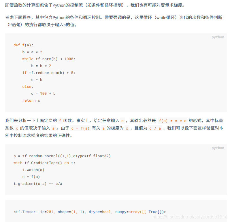
3.4 高阶导数

在 ‘GradientTape’ 上下文管理器中记录的操作会用于自动微分。如果导数是在上下文中计算的，导数的函数也会被记录下来。因此，同个 API 可以用于高阶导数。例如：

x = tf.Variable(1.0) # Create a Tensorflow variable initialized to 1.0 with tf.GradientTape() as t: with tf.GradientTape() as t2: y = x * x * x # Compute the gradient inside the 't' context manager # which means the gradient computation is differentiable as well. dy_dx = t2.gradient(y, x) d2y_dx2 = t.gradient(dy_dx, x) assert dy_dx.numpy() == 3.0 assert d2y_dx2.numpy() == 6.0 

精彩推荐：
最全Tensorflow2.0 入门教程持续更新
tensorflow官方教程