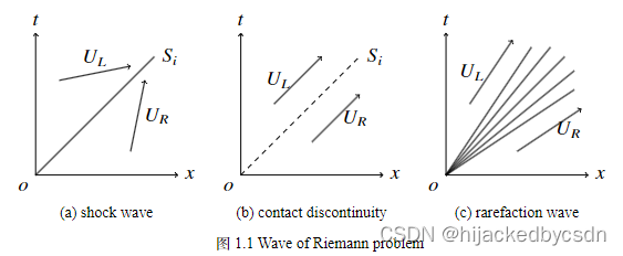
1. 三种膨胀波

Latex 代码

\begin{figure} \centering \begin{subfigure}[b]{0.32\textwidth} \centering \resizebox{\linewidth}{!}{ \begin{tikzpicture} \coordinate (o) at (0,0); \coordinate (S1) at (2.5,2.5); \draw[->] (0,0) -- (3,0) node[right] {$x$}; \draw[->] (0,0) -- (0,3) node[above] {$t$}; \draw[-] (o) -- (S1) node[right] {$S_1$}; \draw[->] (0.5,2) -- (2,2.3) node[midway, above] {$\boldsymbol{U}_L$}; \draw[->] (2,0.5) -- (2.3,2) node[midway, right] {$\boldsymbol{U}_R$}; \node[below left] {$o$}; \end{tikzpicture} } \caption{shock wave} \label{fig:shock_wave_1} \end{subfigure} \begin{subfigure}[b]{0.32\textwidth} \centering \resizebox{\linewidth}{!}{ \begin{tikzpicture} \coordinate (o) at (0,0); \coordinate (S2) at (2.5,2.5); \draw[->] (0,0) -- (3,0) node[right] {$x$}; \draw[->] (0,0) -- (0,3) node[above] {$t$}; \draw[dashed] (o) -- (S2) node[right] {$S_2$}; \draw[->] (0.7,1.5) -- (1.7,2.5) node[midway, left] {$\boldsymbol{U}_L$}; \draw[->] (1.5,0.7) -- (2.5,1.7) node[midway, right] {$\boldsymbol{U}_R$}; \node[below left] {$o$}; \end{tikzpicture} } \caption{contact discontinuity} \label{fig:contact_discontinuity_1} \end{subfigure} \begin{subfigure}[b]{0.32\textwidth} \centering \resizebox{\linewidth}{!}{ \begin{tikzpicture} \coordinate (o) at (0,0); \coordinate (S1) at (1.8,2.7); \coordinate (S2) at (2.2,2.7); \coordinate (S3) at (2.5,2.5); \coordinate (S4) at (2.7,2.2); \coordinate (S5) at (2.7,1.8); \draw[->] (0,0) -- (3,0) node[right] {$x$}; \draw[->] (0,0) -- (0,3) node[above] {$t$}; \draw[-] (o) -- (S1) node[right] {}; \draw[-] (o) -- (S2) node[right] {}; \draw[-] (o) -- (S3) node[right] {}; \draw[-] (o) -- (S4) node[right] {}; \draw[-] (o) -- (S5) node[right] {}; \draw[->] (0.5,1.5) -- (1.4,2.85) node[midway, left] {$\boldsymbol{U}_L$}; \draw[->] (1.5,0.5) -- (2.85,1.4) node[midway, right] {$\boldsymbol{U}_R$}; \node[below left] {$o$}; \end{tikzpicture} } \caption{rarefaction wave} \label{fig:rarefaction_wave_1} \end{subfigure} \caption{Wave of Riemann problem. $S_1, S_2$ is wave speed, $U_L,U_R$ are initial data states connected by a single wave.} \label{fig:wave_of_riemann} \end{figure} 

输出：

讯享网

绘图参考：

《Riemann Solvers and Numerical Methods for Fluid Dynamics》P84

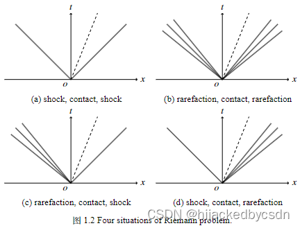
2. Riemann 问题的解

Latex 代码：

讯享网\begin{figure} \centering \begin{subfigure}[b]{0.4\textwidth} \centering \resizebox{\linewidth}{!}{ \begin{tikzpicture} \coordinate (o) at (0,0); \coordinate (S1) at (2.5,2.5); \coordinate (S2) at (1.2,3); \coordinate (S3) at (-2.5,2.5); \draw[->] (-3,0) -- (3,0) node[right] {$x$}; \draw[->] (0,0) -- (0,3) node[above] {$t$}; \draw[-] (o) -- (S1) node[right] {}; \draw[dashed] (o) -- (S2) node[right] {}; \draw[-] (o) -- (S3) node[right] {}; \node[below left] (o) {$o$}; \end{tikzpicture} } \caption{shock, contact, shock} \label{fig:riemann_sol_1} \end{subfigure} \begin{subfigure}[b]{0.4\textwidth} \centering \resizebox{\linewidth}{!}{ \begin{tikzpicture} \coordinate (o) at (0,0); \coordinate (S1) at (2.2,2.7); \coordinate (S2) at (2.5,2.5); \coordinate (S3) at (2.7,2.2); \coordinate (S4) at (1.2,3); \coordinate (S5) at (-2.2,2.7); \coordinate (S6) at (-2.5,2.5); \coordinate (S7) at (-2.7,2.2); \draw[->] (-3,0) -- (3,0) node[right] {$x$}; \draw[->] (0,0) -- (0,3) node[above] {$t$}; \draw[-] (o) -- (S1) node[right] {}; \draw[-] (o) -- (S2) node[right] {}; \draw[-] (o) -- (S3) node[right] {}; \draw[dashed] (o) -- (S4) node[right] {}; \draw[-] (o) -- (S5) node[right] {}; \draw[-] (o) -- (S6) node[right] {}; \draw[-] (o) -- (S7) node[right] {}; \node[below left] (o) {$o$}; \end{tikzpicture} } \caption{rarefaction, contact, rarefaction} \label{fig:riemann_sol_2} \end{subfigure}\\ \begin{subfigure}[b]{0.4\textwidth} \centering \resizebox{\linewidth}{!}{ \begin{tikzpicture} \coordinate (o) at (0,0); \coordinate (S1) at (2.5,2.5); \coordinate (S2) at (1.2,3); \coordinate (S3) at (-2.2,2.7); \coordinate (S4) at (-2.5,2.5); \coordinate (S5) at (-2.7,2.2); \draw[->] (-3,0) -- (3,0) node[right] {$x$}; \draw[->] (0,0) -- (0,3) node[above] {$t$}; \draw[-] (o) -- (S1) node[right] {}; \draw[dashed] (o) -- (S2) node[right] {}; \draw[-] (o) -- (S3) node[right] {}; \draw[-] (o) -- (S4) node[right] {}; \draw[-] (o) -- (S5) node[right] {}; \node[below left] (o) {$o$}; \end{tikzpicture} } \caption{rarefaction, contact, shock} \label{fig:riemann_sol_3} \end{subfigure} \begin{subfigure}[b]{0.4\textwidth} \centering \resizebox{\linewidth}{!}{ \begin{tikzpicture} \coordinate (o) at (0,0); \coordinate (S1) at (2.2,2.7); \coordinate (S2) at (2.5,2.5); \coordinate (S3) at (2.7,2.2); \coordinate (S4) at (1.2,3); \coordinate (S5) at (-2.5,2.5); \draw[->] (-3,0) -- (3,0) node[right] {$x$}; \draw[->] (0,0) -- (0,3) node[above] {$t$}; \draw[-] (o) -- (S1) node[right] {}; \draw[-] (o) -- (S2) node[right] {}; \draw[-] (o) -- (S3) node[right] {}; \draw[dashed] (o) -- (S4) node[right] {}; \draw[-] (o) -- (S5) node[right] {}; \node[below left] (o) {$o$}; \end{tikzpicture} } \caption{shock, contact, rarefaction} \label{fig:riemann_sol_4} \end{subfigure} \caption{Four situations of Riemann problem.} \label{fig:riemann_four_solutions} \end{figure} 

输出：

绘图参考：

《Riemann Solvers and Numerical Methods for Fluid Dynamics》P118