卷积神经网络模型

大家好，我是讯享网，很高兴认识大家。

引言：

1.LeNet

2.AlexNet

3.VGG

4.GoogleNet

5.ResNet

6.DenseNet

7.总结

引言：

在深度学习中，卷积神经网络（CNN）在计算机视觉领域的应用十分广泛。本文章旨在介绍一些CNN的模型，并分析各自模型的优缺点。

1.LeNet

LeNet模型是在1998年提出的一种图像分类模型，应用于支票或邮件编码上的手写数字的识别，也被认为是最早的卷积神经网络(CNN)，为后续CNN的发展奠定了基础，作者LeCun Y也被誉为卷积神经网络之父。

LeNet分为卷积层和全连接层。在卷积层中卷积运算提取输入数据的特征，在卷积层之后会将结果送入激活函数，激活函数会将结果进行非线性的变换，解决线性模型表达能力不足的缺陷，然后会将激活函数的输出送入池化层，对特征进行挑选，降低卷积层对位置的敏感性。下图为LeNet的网络结构图。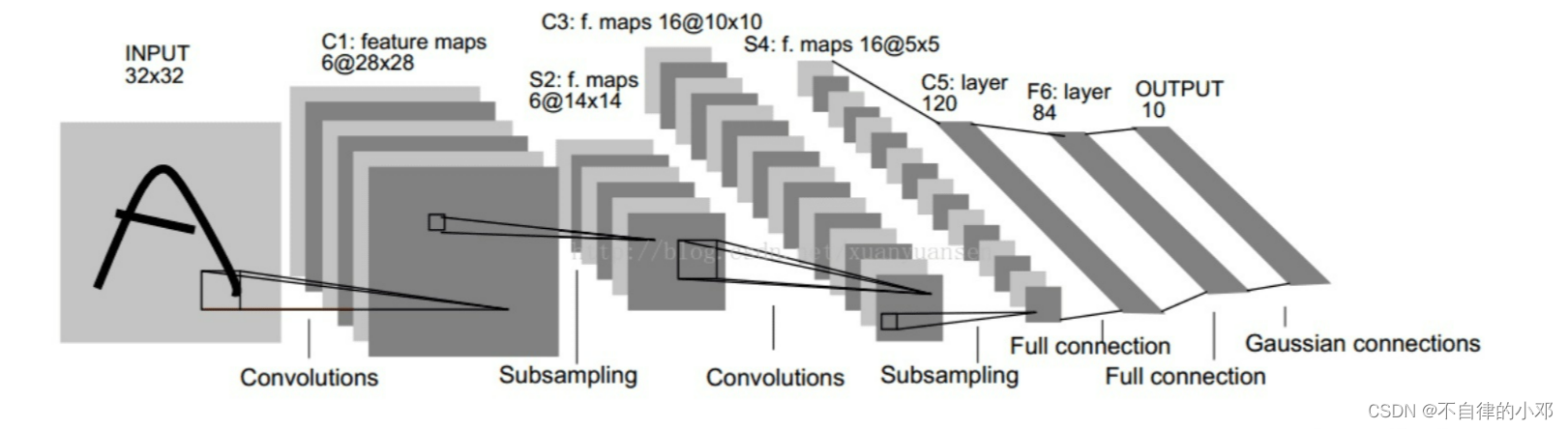
讯享网

从网络结构图就能够知道LeNet有以下特点：

1）网络结构简单，容易实现。LeNet只有两个卷积层，两个池化层，三个全连接层，层与层之间又加入了激活函数。

2）小尺寸输入。LeNet的输入只有32×32的大小，这与现在许多网络输入相比，显得小了很多。

下面用Pytorch来写LeNet的代码：

①数据加载：

import sys from torchvision.transforms import transforms,ToTensor import torch import torch.nn as nn import torch.nn.functional as F import torchvision import time mnist_train = torchvision.datasets.FashionMNIST(root='~/Datasets/FashionMNIST', train=True, download=True, transform=transforms.ToTensor()) mnist_test = torchvision.datasets.FashionMNIST(root='~/Datasets/FashionMNIST', train=False, download=True, transform=transforms.ToTensor()) def load_data_fashion_mnist(mnist_train, mnist_test, batch_size): if sys.platform.startswith('win'): num_workers = 0 else: num_workers = 4 train_iter = torch.utils.data.DataLoader(mnist_train, batch_size=batch_size, shuffle=True, num_workers=num_workers) test_iter = torch.utils.data.DataLoader(mnist_test, batch_size=batch_size, shuffle=False, num_workers=num_workers) return train_iter, test_iter batch_size = 256 train_iter, test_iter = load_data_fashion_mnist(mnist_train, mnist_test, batch_size)

讯享网

②网络构建：

讯享网class LeNet(nn.Module): def __init__(self): super(LeNet, self).__init__() self.conv = nn.Sequential( nn.Conv2d(1,6,5), nn.Sigmoid(), nn.MaxPool2d(2,2), nn.Conv2d(6,16,5), nn.Sigmoid(), nn.MaxPool2d(2,2) ) self.fc = nn.Sequential( nn.Linear(16*4*4,120), nn.Sigmoid(), nn.Linear(120,84), nn.Sigmoid(), nn.Linear(84,10), ) def forward(self, x): feature = self.conv(x) output = self.fc(feature.view(x.shape[0], -1)) return output

③模型训练及预测：

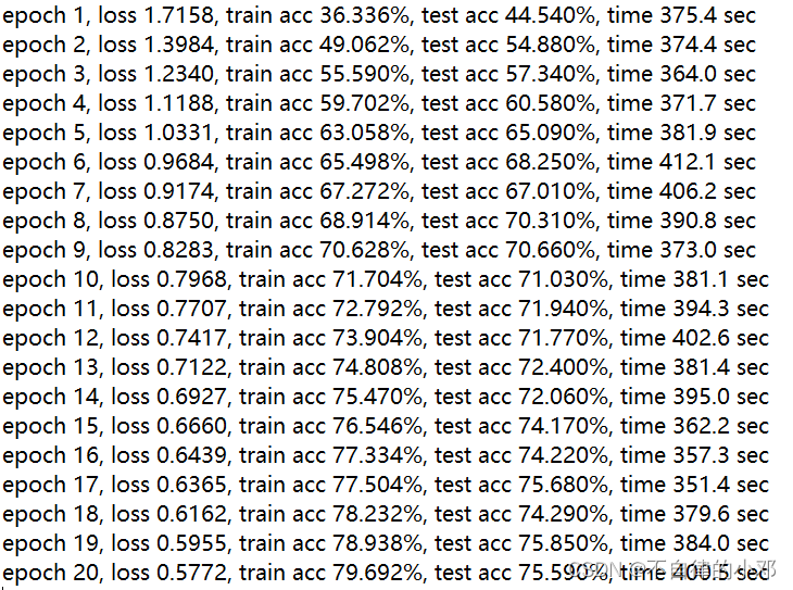
net = LeNet() device = torch.device('cuda:3' if torch.cuda.is_available() else 'cpu') def evaluate_accuracy(iter,net,device=None): if device is None and isinstance(net,torch.nn.Module): device = list(net.parameters())[0].device acc_sum,n = 0.0,0 with torch.no_grad(): for x,y in iter: net.eval() acc_sum += (net(x.to(device)).argmax(dim=1)==y.to(device)).float().sum().cpu().item() net.train() n += y.shape[0] return acc_sum/n def train(net,train_iter,test_iter,batch_size,optimizer,device,num_epochs): net = net.to(device) print("training on ", device) loss = nn.CrossEntropyLoss() for epoch in range(num_epochs): train_l_sum, train_acc_sum, n, batch_count, start = 0.0, 0.0, 0, 0, time.time() for x, y in train_iter: x = x.to(device) y = y.to(device) y_hat = net(x) l = loss(y_hat,y) optimizer.zero_grad() l.backward() optimizer.step() train_l_sum += l.cpu().item() train_acc_sum += (y_hat.argmax(dim=1) == y).sum().cpu().item() n += y.shape[0] batch_count += 1 test_acc = evaluate_accuracy(test_iter, net) print('epoch %d, loss %.4f, train acc %.3f, test acc %.3f, time %.1f sec' % (epoch + 1, train_l_sum / batch_count, train_acc_sum / n, test_acc, time.time() - start)) lr, num_epochs = 0.001, 20 optimizer = torch.optim.Adam(net.parameters(), lr=lr) train(net, train_iter, test_iter, batch_size, optimizer, device, num_epochs)

④运行结果：

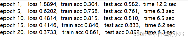
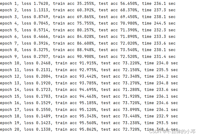
从运行结果可以看出，LeNet的损失稳定下降，准确率逐渐提高，并且运行时间也逐渐减少。这表明LeNet模型的训练过程是有效的，模型在不断学习并提高性能。

从代码可以看出，LeNet的网络组成简单，易于实现，参数少，容易扩展。但是缺点也很明显，它对于复杂情况的处理能力欠缺，且精度并不是特别高（也有可能是其他的参数影响）。LeNet发明较早，随着卷积神经网络的发展，它对于现今的计算机视觉并不是首选模型。

2.AlexNet

AlexNet由Hinton和他的学生Alex Krizhevsky设计，模型名字来源于论文第一作者的姓名Alex。该模型以很大的优势获得了2012年ISLVRC竞赛的冠军网络，分类准确率由传统的 70%+提升到 80%+。

下面根据Alex net网络结构图对每层进行讲解讲解。

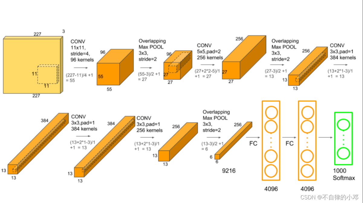
（1）input：输入数据为227*227*3的图像。

（2）conv1：in_channels=1, out_channels=96, kernel_size=11, stride=4, padding=0。

套用卷积公式可得输出数据为： $\frac{227-11}{4}+1=55$ ,输出特征图为55*55*96。

（3）pooling1：kernel_size=3, stride=2。输出的特征图为：27*27*96。

（4）conv2：in_channels=96, out_channels=256, kernel_size=5, stride=1, padding=2。

输出数据为： $\frac{27-5+4}{1}+1=27$ ，输出特征图为27*27*256.

（5）pooling2:kernel_size=3, stride=2。输出的特征图为：13*13*256。

（6）conv3:in_channels=256, out_channels=384, kernel_size=3, stride=1, padding=1。

输出数据为： $\frac{13-3+2}{1}+1=13$ ，输出特征图为13*13*384。

（7）conv4：in_channels=384, out_channels=384, kernel_size=3, stride=1, padding=1。

输出数据为： $\frac{13-3+2}{1}+1=13$ ，输出特征图为13*13*384。

（8）conv4：in_channels=384, out_channels=256, kernel_size=3, stride=1, padding=1。

输出数据为： $\frac{13-3+2}{1}+1=13$ ，输出特征图为13*13*256。

（9）pooling3：pooling2:kernel_size=3, stride=2。输出的特征图为：6*6*256。

（10）FC1：是AlexNet的第一个全连接层，输入为5*5*256，输出为1*4096。

（11）FC2：AlexNet的第二个全连接层，输入为1*4096，输出为1*4096。

（12）FC3：AlexNet的第三个全连接层，输入为1*4096，输出为1*10。

在理解完AlexNet的网络结构以后，可以看出AlexNet有如下几个特点：

1）较深的网络结构。有五个卷积层，三个池化层，三个全连接层，相比于LeNet有着更好的学习能力。

2）使用了ReLu激活函数。ReLu函数有效的解决了梯度消失的问题，并增强了网络的非线性表达能力。

3）采用了Dropout。在前两个全连接层之后会采用Dropout，随机丢弃一部分神经元，减少网络过拟合风险，使得网络的训练过程更加鲁棒。

直接上代码。

①数据加载：

讯享网import time import torch from torch import nn, optim import torchvision import sys device = torch.device('cuda:4' if torch.cuda.is_available() else 'cpu') def load_data_fashion_mnist(batch_size, resize=None, root='./data_FashionMNIST'): if sys.platform.startswith('win'): num_workers = 0 else: num_workers = 4 trans = [] if resize: trans.append(torchvision.transforms.Resize(size=resize)) trans.append(torchvision.transforms.ToTensor()) transform = torchvision.transforms.Compose(trans) mnist_train = torchvision.datasets.FashionMNIST(root=root, train=True, download=True, transform=transform) mnist_test = torchvision.datasets.FashionMNIST(root=root, train=False, download=True, transform=transform) train_iter = torch.utils.data.DataLoader(mnist_train, batch_size=batch_size, shuffle=True, num_workers=num_workers) test_iter = torch.utils.data.DataLoader(mnist_test, batch_size=batch_size, shuffle=False, num_workers=num_workers) return train_iter, test_iter batch_size = 128 train_iter, test_iter = load_data_fashion_mnist(batch_size, resize=224)

②构建网络：

class AlexNet(nn.Module): def __init__(self): super(AlexNet, self).__init__() self.conv = nn.Sequential( nn.Conv2d(1, 96, 11, 4), # in_channels, out_channels, kernel_size, stride, padding nn.ReLU(), nn.MaxPool2d(3, 2), # kernel_size, stride # 减小卷积窗口，使用填充为2来使得输入与输出的高和宽一致，且增大输出通道数 nn.Conv2d(96, 256, 5, 1, 2), nn.ReLU(), nn.MaxPool2d(3, 2), # 连续3个卷积层，且使用更小的卷积窗口。除了最后的卷积层外，进一步增大了输出通道数。 nn.Conv2d(256, 384, 3, 1, 1), nn.ReLU(), nn.Conv2d(384, 384, 3, 1, 1), nn.ReLU(), nn.Conv2d(384, 256, 3, 1, 1), nn.ReLU(), nn.MaxPool2d(3, 2) ) self.fc = nn.Sequential( nn.Linear(256*5*5, 4096), nn.ReLU(), nn.Dropout(0.5), nn.Linear(4096, 4096), nn.ReLU(), nn.Dropout(0.5), nn.Linear(4096, 10), ) def forward(self, img): feature = self.conv(img) output = self.fc(feature.view(img.shape[0], -1)) return output

③模型训练及预测：

讯享网net = AlexNet() def evaluate_accuracy(data_iter, net, device=None): if device is None and isinstance(net, torch.nn.Module): # 如果没指定device就使用net的device device = list(net.parameters())[0].device acc_sum, n = 0.0, 0 with torch.no_grad(): for X, y in data_iter: net.eval() # 评估模式, 这会关闭dropout acc_sum += (net(X.to(device)).argmax(dim=1) == y.to(device)).float().sum().cpu().item() net.train() # 改回训练模式 n += y.shape[0] return acc_sum / n def train(net, train_iter, test_iter, batch_size, optimizer, device, num_epochs): net = net.to(device) print("training on ", device) loss = torch.nn.CrossEntropyLoss() for epoch in range(num_epochs): train_l_sum, train_acc_sum, n, batch_count, start = 0.0, 0.0, 0, 0, time.time() for X, y in train_iter: X = X.to(device) y = y.to(device) y_hat = net(X) l = loss(y_hat, y) optimizer.zero_grad() l.backward() optimizer.step() train_l_sum += l.cpu().item() train_acc_sum += (y_hat.argmax(dim=1) == y).sum().cpu().item() n += y.shape[0] batch_count += 1 test_acc = evaluate_accuracy(test_iter, net) print('epoch %d, loss %.4f, train acc %.3f, test acc %.3f, time %.1f sec' % (epoch + 1, train_l_sum / batch_count, train_acc_sum / n, test_acc, time.time() - start)) lr, num_epochs = 0.001, 20 optimizer = torch.optim.Adam(net.parameters(), lr=lr) train(net, train_iter, test_iter, batch_size, optimizer, device, num_epochs)

④运行结果：

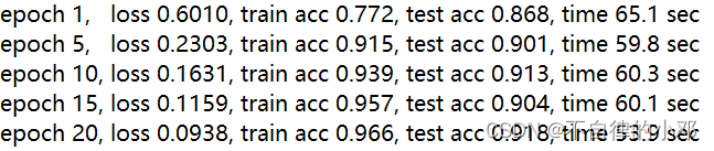
运行结果相较于LeNet来说，loss值函数逐渐减小，并比LeNe的losst小很多，AlexNet在训练集准确率比LeNet高10%左右，在测试集高5%，但是每训练一个epoch所花费的时间也比LeNet高很多。

从代码实现上来看，AlexNet网络更加复杂，层数更多，而且使用了三个全连接层。这使得AlexNet在处理复杂的问题时具有更强的建模能力和表达能力。然而，由于网络的复杂性，训练AlexNet模型可能需要更长的时间和更多的计算资源。因此，在处理简单的图像问题时，LeNet模型可能已经足够有效，而在面对更复杂的问题时，AlexNet可以发挥其优势。

3.VGG

VGG是2014年Oxford的Visual Geometry Group提出的，其在在2014年的 ImageNet 大规模视觉识别挑(ILSVRC -2014中获得了亚军，第一名是GoogleNet。该网络是作者参加ILSVRC 2014比赛上的作者所做的相关工作，相比AlexNet，VGG使用了更深的网络结构，证明了增加网络深度能够在一定程度上影响网络性能。

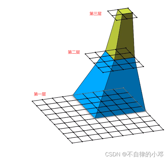
VGG的核心思想是通过增加网络模型的深度来提高模型的性能。VGG使用了相同大小的卷积核以及池化层，例如使用3×3的卷积核，2×2的池化窗口。利用相同大小的卷积块代替卷积核较大的卷积块，既能够减少网络参数，又可以拥有相同大小的感受野。那什么是感受野呢？在卷积神经网络中，决定一个输出结果中一个元素所对应的输入层的区域大小，被称为感受野。也就相当于这一层的一个单元对应在上一层（输入层）所占的区域大小。感受野的计算公式： $F(i) = (F(i+1) - 1) \times stride + kernel$

可以根据下图来更好的理解什么是感受野。第三层的1个单元格，对应第二层的感受野为2×2个单元格，对应第一层的5×5个单元格。

VGG网络配置：

根据卷积核的大小核卷积层数，VGG共有6种配置，分别为A、A-LRN、B、C、D、E，其中D和E就是最为常用的VGG16和VGG19。

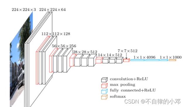
介绍结构图：

在这里插入图片描述

conv3-64 ：是指第三层卷积后维度变成64，同样，conv3-128指的是第三层卷积后维度变成128。
input（224x224 RGB image）：指的是输入图片大小为224*224*3。
maxpool ：是指最大池化，在vgg16中，pooling采用的是2*2的最大池化方法。
FC-4096 :指的是全连接层中有4096个节点，FC-1000为该层全连接层有1000个节点。
padding：指的是对矩阵在外边填充n圈，padding=1即填充1圈，5X5大小的矩阵，填充一圈后变成7X7大小。
vgg16每层卷积的滑动步长stride=1，padding=1，卷积核大小为3*3。

VGG网络的卷积块和池化窗口的大小都是一样的，所以写VGG网络时不用去定义卷积层和池化层，只需要调用存储了VGG卷积层和池化层配置的‘cfg’，并通过函数将卷积层和池化层定义出来即可。以VGG16为例，输入的数据为224×224×3，卷积核大小为3×3，池化窗口大小为2×2，根据卷积公式： $W_{output}=\frac{W_{input}-W_{kernel}+2Padding}{stride}+1$ 就可以计算出每一层输出数据的大小，这里就不再做运算。

综上所述，我们可以得出VGG有以下特点：

1）网络结构简单。VGG的网络结构简单在它只会有3×3的卷积层，以及2×2的池化层，使得网络的结构十分简单，容易理解。

2）VGG采用了小卷积核代替大卷积核。VGG16采用的是两个3×3卷积核替代5×5卷积核的策略，减少了网络的参数量，降低了过拟合的风险。

3）深度网络结构的使用。VGG最多可以堆叠到19层，通过堆叠卷积块和池化窗口，使模型能够提取出更加丰富的特征，并且提高了对复杂情况的处理能力，从而提高了对图片分类和识别的准确性。

①加载数据：

import time import torchvision.datasets from torch.utils.data import DataLoader from torchvision import transforms from torchvision.datasets import CIFAR10 from VGG import * from torchvision.transforms import Compose,Normalize,Resize,ToTensor,Grayscale batch_size = 32 device = torch.device('cuda:0' if torch.cuda.is_available() else 'cpu') def CIFAR10_loader(size,train=True): transform_fn = Compose([ Resize((size,size)), ToTensor(), Normalize(mean=[0.485,0.456,0.406],std=[0.229,0.224,0.225]) ]) dataset = CIFAR10(root='../CIFAR10', train=train, transform=transform_fn, download=True) data_loader = DataLoader(dataset,batch_size=32,shuffle=True) return data_loader train_dataloader = CIFAR10_loader(size=224,train=True) test_dataloader = CIFAR10_loader(size=224,train=False) model = vgg('vgg11')

②构建网络模型：

讯享网import torch.nn as nn import torch model_urls = { 'vgg11': 'https://download.pytorch.org/models/vgg11-bbd30ac9.pth', 'vgg13': 'https://download.pytorch.org/models/vgg13-ca.pth', 'vgg16': 'https://download.pytorch.org/models/vgg16-af.pth', 'vgg19': 'https://download.pytorch.org/models/vgg19-dcbb9e9d.pth' } class VGG(nn.Module): def __init__(self, features, num_classes=10, init_weights=False): super(VGG, self).__init__() self.features = features self.classifier = nn.Sequential( nn.Linear(512 * 7 * 7, 4096), nn.ReLU(True), nn.Dropout(p=0.5), nn.Linear(4096, 4096), nn.ReLU(True), nn.Dropout(p=0.5), nn.Linear(4096, num_classes) ) if init_weights: self._initialize_weights() def forward(self, x): x = self.features(x) x = torch.flatten(x, start_dim=1) x = self.classifier(x) return x def _initialize_weights(self): for m in self.modules(): if isinstance(m, nn.Conv2d): nn.init.xavier_uniform_(m.weight) if m.bias is not None: nn.init.constant_(m.bias, 0) elif isinstance(m, nn.Linear): nn.init.xavier_uniform_(m.weight) nn.init.constant_(m.bias, 0) def make_features(cfg: list): #卷积块 layers = [] in_channels = 3 for v in cfg: if v == "M": layers += [nn.MaxPool2d(kernel_size=2, stride=2)] else: conv2d = nn.Conv2d(in_channels, v, kernel_size=3, padding=1) layers += [conv2d, nn.ReLU(True)] in_channels = v return nn.Sequential(*layers) cfgs = { 'vgg11': [64, 'M', 128, 'M', 256, 256, 'M', 512, 512, 'M', 512, 512, 'M'], 'vgg13': [64, 64, 'M', 128, 128, 'M', 256, 256, 'M', 512, 512, 'M', 512, 512, 'M'], 'vgg16': [64, 64, 'M', 128, 128, 'M', 256, 256, 256, 'M', 512, 512, 512, 'M', 512, 512, 512, 'M'], 'vgg19': [64, 64, 'M', 128, 128, 'M', 256, 256, 256, 256, 'M', 512, 512, 512, 512, 'M', 512, 512, 512, 512, 'M'], } def vgg(model_name="vgg16", kwargs): assert model_name in cfgs, "Warning: model number {} not in cfgs dict!".format(model_name) cfg = cfgs[model_name] model = VGG(make_features(cfg), kwargs) return model

③模型的训练及测试：

in_channels = 1 model = vgg('vgg11') def evaluate_accuracy(data_iter, net, device=None): if device is None and isinstance(net, torch.nn.Module): device = list(net.parameters())[0].device acc_sum, n = 0.0, 0 with torch.no_grad(): for X, y in data_iter: net.eval() acc_sum += (net(X.to(device)).argmax(dim=1) == y.to(device)).float().sum().cpu().item() net.train() n += y.shape[0] return acc_sum / n def train(net, train_iter, test_iter, batch_size, optimizer, device, num_epochs): net = net.to(device) print("training on ", device) loss = torch.nn.CrossEntropyLoss() for epoch in range(num_epochs): train_l_sum, train_acc_sum, n, batch_count, start = 0.0, 0.0, 0, 0, time.time() for X, y in train_iter: X = X.to(device) y = y.to(device) y_hat = net(X) l = loss(y_hat, y) optimizer.zero_grad() l.backward() optimizer.step() train_l_sum += l.cpu().item() train_acc_sum += (y_hat.argmax(dim=1) == y).sum().cpu().item() n += y.shape[0] batch_count += 1 test_acc = evaluate_accuracy(test_iter, net) print('epoch %d, loss %.4f, train acc %.3f%%, test acc %.3f%%, time %.1f sec' % (epoch + 1, train_l_sum / batch_count, 100*train_acc_sum / n, 100*test_acc, time.time() - start)) iteration = 10000 num_epochs = 20 learning_rate = 0.001 optimizer = torch.optim.Adam(model.parameters(), lr=learning_rate) train(model, train_dataloader, test_dataloader, batch_size, optimizer, device, num_epochs)

④预测结果：

数据集采用的是CIFAR10，数据集较小采用的是VGG11，batch_size=32，当把batch_size调的较小时，结果的准确率会一直维持在10%左右，可能是发生了梯度消失。从结果可以看出在训练集的准确率远远大于测试集的准确率，并且测试集的准确率到了第5个epoch开始就维持在72%左右，这就说明发生了过拟合的现象，可能是没用正则化的方法，也可能是因为VGG16的模型过大，采用CIFAR10较小的数据集，数据量可能不足以让模型充分学习。训练只运行了20个epoch，并且将batch_size为8，运行时间平均都在300s，VGG模型所需要的资源以及时间耗费都是比较大的。

相较于LeNet和AlexNet，VGG的模型深度更深，并且参数量也更大，更适合处理复杂任务，但是它所需要的计算资源和训练时间较大，并且在使用小数据集时，可能会发生过拟合的情况，需要根据自己的具体情况再考虑是否需要用到VGG。

4.GoogleNet

VGG结构是通过增加深度使得网络获得更好的性能(纵向)，那可不可以通过拓宽网络的宽度(横向)，使得网络也能够有更好的性能呢？答案是肯定的，GoogleNet就是这样做，并且获得了2014年ImageNet竞赛的冠军。

GoogleNet的核心是它采用了Inception模块提取图片的特征，从而让GoogleNet在横向扩展了网络。

Inception模块：

左边的图片，猫的图像占了绝大部分，而在右边的猫只有50%左右，尺寸较大的卷积核适合全局分布的特征提取，较小的卷积核适合提取局部特征，但是如果简单的将两者堆叠，会提高参数量以及计算量，并且较深的网络容易过拟合。接下来看Inception的网络结构图。

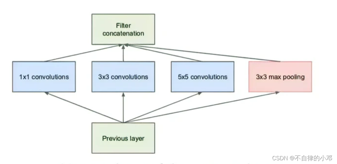
输入数据后，会将数据送入三个滤波器和一个池化窗口中，滤波器有1×1，3×3，5×5相比于单一的滤波器，提取的特征更加丰富。最后将四个的输出一并输入到下一个Inception模块中。

带降维的Inception模块：

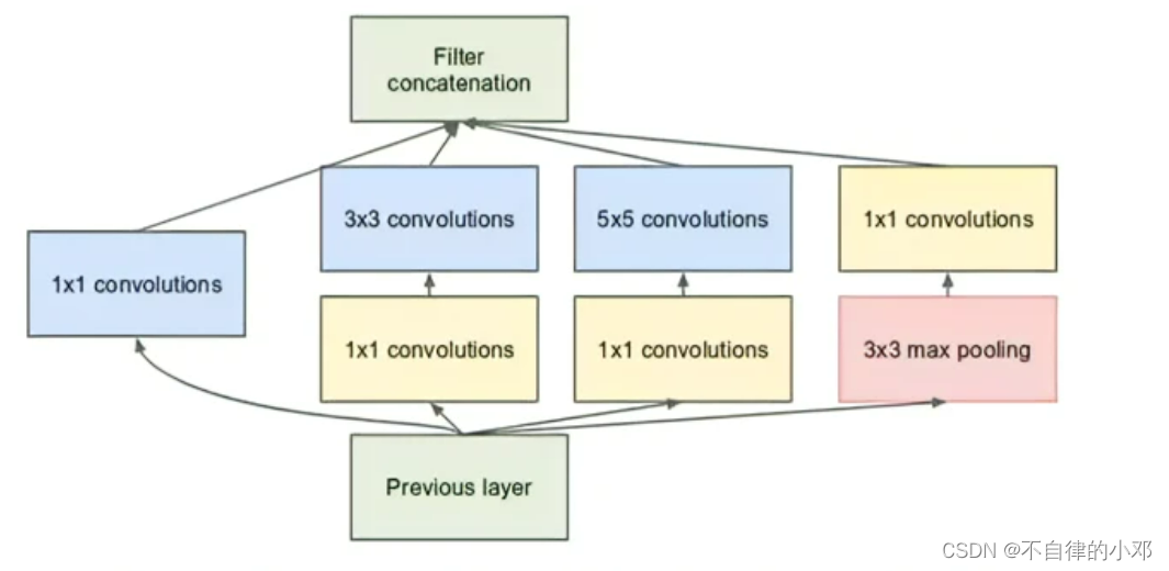
带降维的Inception模块变化不大，在3×3，5×5卷积之前，池化之后分别加入了一个1×1的卷积核，这个卷积核是为了改变通道数，并不改变数据大小。在减少通道数后，网络的参数也就会减少。

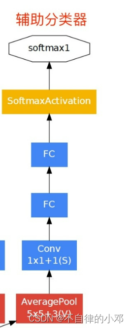
辅助分类器：

在GoogleNet中引入了两个辅助分类器，这两个辅助分类器的作用是避免梯度消失，用于向前传导梯度，也有一定的正则化效果，防止过拟合。

给出的代码为没有加辅助分类器的代码：

①构建网络：

讯享网import torch from torch import nn from torch.nn import functional as F class Inception(nn.Module): def __init__(self, in_channels, c1, c2, c3, c4,): super(Inception, self).__init__() self.p1_1 = nn.Conv2d(in_channels, c1, kernel_size=1) self.p2_1 = nn.Conv2d(in_channels, c2[0], kernel_size=1) self.p2_2 = nn.Conv2d(c2[0], c2[1], kernel_size=3, padding=1) self.p3_1 = nn.Conv2d(in_channels, c3[0], kernel_size=1) self.p3_2 = nn.Conv2d(c3[0], c3[1], kernel_size=5, padding=2) self.p4_1 = nn.MaxPool2d(kernel_size=3, stride=1, padding=1) self.p4_2 = nn.Conv2d(in_channels, c4, kernel_size=1) def forward(self, x): p1 = F.relu(self.p1_1(x)) p2 = F.relu(self.p2_2(F.relu(self.p2_1(x)))) p3 = F.relu(self.p3_2(F.relu(self.p3_1(x)))) p4 = F.relu(self.p4_2(self.p4_1(x))) return torch.cat((p1, p2, p3, p4), dim=1) class GoogLeNet(nn.Module): def __init__(self, in_channels=3, num_classes=10): super(GoogLeNet, self).__init__() # 第一阶段 self.stage1 = nn.Sequential( nn.Conv2d(in_channels, 64, kernel_size=7, stride=2, padding=3), nn.ReLU(inplace=True), nn.MaxPool2d(kernel_size=3, stride=2, padding=1) ) # 第二阶段 self.stage2 = nn.Sequential( nn.Conv2d(64, 64, kernel_size=1), nn.ReLU(inplace=True), nn.Conv2d(64, 192, kernel_size=3, padding=1), nn.ReLU(inplace=True), nn.MaxPool2d(kernel_size=3, stride=2, padding=1) ) # 第三阶段 self.stage3 = nn.Sequential( Inception(in_channels=192, c1=64, c2=(96, 128), c3=(16, 32), c4=32), Inception(256, 128, (128, 192), (32, 96), 64), nn.MaxPool2d(kernel_size=3, stride=2, padding=1) ) # 第四阶段 self.stage4 = nn.Sequential( Inception(480, 192, (96, 208), (16, 48), 64), Inception(512, 160, (112, 224), (24, 64), 64), Inception(512, 128, (128, 256), (24, 64), 64), Inception(512, 112, (144, 288), (32, 64), 64), Inception(528, 256, (160, 320), (32, 128), 128), nn.MaxPool2d(kernel_size=3, stride=2, padding=1) ) # 第五阶段 self.stage5 = nn.Sequential( Inception(832, 256, (160, 320), (32, 128), 128), Inception(832, 384, (192, 384), (48, 128), 128), nn.AdaptiveAvgPool2d((1, 1)), nn.Flatten() ) # 全连接层 self.fc = nn.Linear(1024, num_classes) def forward(self, x): x = self.stage1(x) x = self.stage2(x) x = self.stage3(x) x = self.stage4(x) x = self.stage5(x) x = self.fc(x) return x

②加载数据和训练模型：

import time from torchvision.transforms import Compose,Normalize,Resize,ToTensor from torchvision.datasets import CIFAR10 from torch.utils.data import DataLoader from GoogleNet import * from torchvision import transforms device = torch.device('cuda:1' if torch.cuda.is_available() else 'cpu') batch_size = 16 def CIFAR10_loader(size,train=True): transform_fn = Compose([ Resize((size,size)), ToTensor(), Normalize(mean=[0.485,0.456,0.406],std=[0.229,0.224,0.225]), ]) dataset = CIFAR10(root='../CIFAR10', train=train, transform=transform_fn, download=True) data_loader = DataLoader(dataset,batch_size=batch_size,shuffle=True) return data_loader train_dataloader = CIFAR10_loader(size=256,train=True) test_dataloader = CIFAR10_loader(size=256,train=False) def evaluate_accuracy(data_iter, net, device=None): if device is None and isinstance(net, torch.nn.Module): device = list(net.parameters())[0].device acc_sum, n = 0.0, 0 with torch.no_grad(): for X, y in data_iter: net.eval() acc_sum += (net(X.to(device)).argmax(dim=1) == y.to(device)).float().sum().cpu().item() net.train() n += y.shape[0] return acc_sum / n def train(net, train_iter, test_iter, loss, optimizer, device,epochs): net = net.to(device) print("training on ", device) batch_count = 0 for epoch in range(epochs): train_l_sum, train_acc_sum, n, start = 0.0, 0.0, 0, time.time() for X, y in train_iter: X, y = X.to(device), y.to(device) y_hat = net(X) l = loss(y_hat, y) optimizer.zero_grad() l.backward() optimizer.step() train_l_sum += l.cpu().item() train_acc_sum += (y_hat.argmax(dim=1) == y).sum().cpu().item() n += y.shape[0] batch_count += 1 test_acc = evaluate_accuracy(test_iter, net, device) print('epoch %d, loss %.4f, train acc %.3f%%, test acc %.3f%%, time %.1f sec' % (epoch + 1, train_l_sum / batch_count, 100 * train_acc_sum / n, 100 * test_acc, time.time() - start)) net = GoogLeNet(num_classes=10) num_epochs = 30 learning_rate = 0.001 optimizer = torch.optim.Adam(net.parameters(), lr=learning_rate) loss = nn.CrossEntropyLoss() train(net, train_dataloader, test_dataloader, loss, optimizer, device, num_epochs)

③预测结果：

epoch 1, loss 2.0922, train acc 19.626%, test acc 36.620%, time 254.4 sec
epoch 2, loss 0.7739, train acc 42.542%, test acc 47.350%, time 257.6 sec
epoch 3, loss 0.4256, train acc 53.686%, test acc 57.690%, time 256.8 sec
epoch 4, loss 0.2726, train acc 60.734%, test acc 61.190%, time 253.0 sec
epoch 5, loss 0.1955, train acc 65.366%, test acc 66.370%, time 256.3 sec
epoch 6, loss 0.1476, train acc 68.518%, test acc 67.110%, time 253.0 sec
epoch 7, loss 0.1154, train acc 71.638%, test acc 70.040%, time 250.2 sec
epoch 8, loss 0.0924, train acc 73.926%, test acc 71.500%, time 250.0 sec
epoch 9, loss 0.0760, train acc 75.870%, test acc 69.940%, time 248.2 sec
epoch 10, loss 0.0628, train acc 77.996%, test acc 71.750%, time 247.3 sec
epoch 11, loss 0.0524, train acc 79.724%, test acc 70.110%, time 246.7 sec
epoch 12, loss 0.0440, train acc 81.418%, test acc 70.500%, time 247.9 sec
epoch 13, loss 0.0371, train acc 82.804%, test acc 72.970%, time 248.1 sec
epoch 14, loss 0.0317, train acc 84.474%, test acc 72.420%, time 246.1 sec
epoch 15, loss 0.0268, train acc 85.970%, test acc 72.940%, time 245.0 sec
epoch 16, loss 0.0232, train acc 86.966%, test acc 71.860%, time 244.3 sec
epoch 17, loss 0.0197, train acc 87.992%, test acc 72.390%, time 387.9 sec
epoch 18, loss 0.0174, train acc 88.734%, test acc 72.170%, time 344.5 sec
epoch 19, loss 0.0155, train acc 89.536%, test acc 72.780%, time 248.2 sec
epoch 20, loss 0.0135, train acc 90.400%, test acc 73.180%, time 248.0 sec

很容易就能够看出，发生了过拟合。还是因为模型的参数太多，小数据集不足以完整地表示整个数据分布的特征，就相当于没有足够的数据支撑模型的训练。

GoogleNet拓宽深度使得它对于局部以及全局的特征提取，都能够保持一个较高的准确性，并且带降维的Inception模块能够降低计算的次数，根据代码的结果来看，GoogleNet还是比较深的，不适用于小数据集。因此，在需要处理较大的复杂的数据集，并且资源有限的情况下，可以选择GoogleNet。

5.ResNet

ResNet 网络是在 2015年由微软实验室中的何凯明等几位大神提出，斩获当年ImageNet竞赛中分类任务第一名，目标检测第一名。获得COCO数据集中目标检测第一名，图像分割第一名。

学习过VGG网络后，可能会有人认为只要让卷积块和池化窗口不断的堆叠使网络的深度足够深，就能够增加网络提取特征的能力，学习效果也会变的更好。但是通过实验发现，随着神经网络的层数不断增加，层数累计到了一定程度，模型的学习效果却变差了。这就有了ResNet,ResNet采用了BatchNormlization(简称BN)解决了梯度消失或者梯度爆炸，用残差学习解决了模型退化的问题。ResNet是由一些Block组成，这些Block会加上之前的输入作为下一个Block的输出，使得网络可以学习残差（residual）函数，从而更有效地训练深层网络。

那什么是BatchNormlization，直译为中文就是批归一化。我们在数据加载时都会对数据进行归一化，让数据能够更快的收敛，但是在上面几个模型数据加载代码中可以看出，归一化的操作只在数据加载是进行了一次，但是当网络开始训练起来时，参数也会随之发生变换，例如在网络的第二次，网络第二层的输入是由第一层的参数和输入计算得到，再训练过程中，参数会变化，所以必然会导致后面每一层输入数据分布的变化。而BatchNormlization就是为了解决在训练过程中，中间层参数分布发生改变的情况。

BN的四个主要步骤为：

1.对每一个训练批次数据求均值。

2.对每一个训练批次数据求方差。

3.用求得的均值和方差对数据进行归一化，获得（0，1）正态分布。其中 $\varepsilon$ 是避免方差为零的微笑正数。

4.由于 $x^{i}$ 求得归一化后符合标准正态分布，会使 $x^{i}$ 的表达能力下降，所以引入了尺度变换 $\lambda$ 和偏移量 $\beta$ ，这两个会在训练网络时得到，加入这两个量后，增强了模型的灵活性以及表达能力。

可能，到这里，还是不能很好的理解BN到底在干什么，只知道归一化，接下来用两幅图就可以直观的感受到BN的作用。

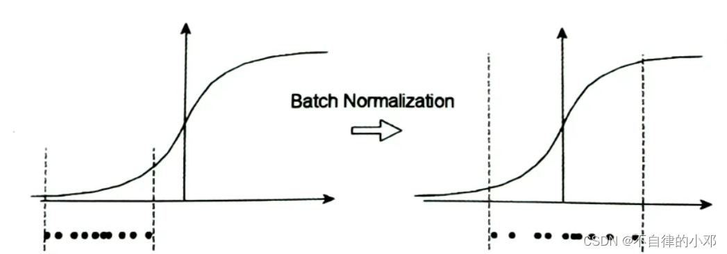
第一幅图表示在为引入BN时，如果数据是在很小的区域，那么学习率很可能就会变慢或者停在某个地方；在加入BN以后，数据均匀的分布在函数的两侧，而这部分大多都是有梯度的，所以，BN是一种能够有效消除梯度消失和梯度爆炸的方法。

那什么是残差(residual)函数？

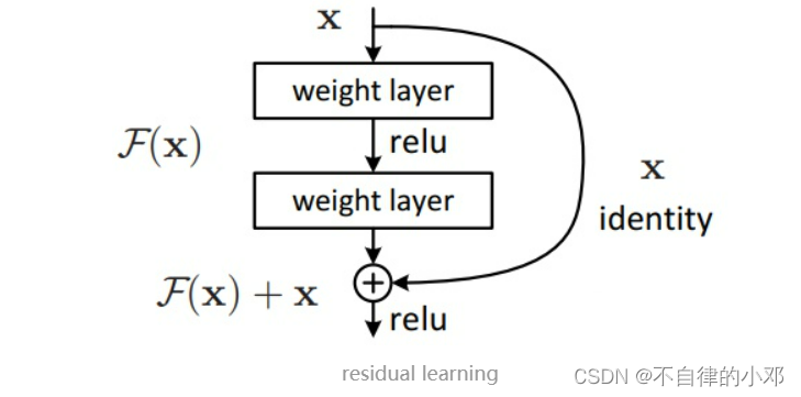
上图可以表达为： H(x) = F (x) + X ，也就是说现在的前向传播函数H(x)为原来的前向传播函数F(x)加上两层之前的输入x。residual结构使用了一种shortcut的连接方式，也可理解为捷径。在ResNet中，有两种相似的残差块，一种叫BasicBlock，另一种叫BottleNeck。

BasicBlock：

在这里插入图片描述

两个3x3的卷积层，通道数都是64，然后就是注意那根跳线，也就是Shortcut Connections，将输入x加到输出。

BottleNeck：

在这里插入图片描述

输入数据先经过1×1的卷积层，通道数由256变为64，再经过3×3的卷积层，最后经过1×1的卷积层，并将通道数从64变为256。1x1卷积层的作用是用于改变特征图的通道数，使得可以和恒等映射x相叠加，另外这里的1x1卷积层改变维度的很重要的一点是可以降低网络参数量，这也是为什么更深层的网络采用BottleNeck而不是BasicBlock的原因。

在这里插入图片描述

由上图可以知道，超过50层的网络，卷积块采用的是BottleNeck。

①加载数据：

讯享网import time import torch.cuda from torchvision.transforms import Compose,Normalize,ToTensor,Resize from torchvision.datasets import CIFAR10 from torch.utils.data import DataLoader from ResNet import * device = torch.device('cuda:3' if torch.cuda.is_available() else 'cpu') batch_size = 128 def CIFAR10_loader(train=True): transform_fn = Compose([ Resize((32,32)), ToTensor(), Normalize(mean=[0.485,0.456,0.406],std=[0.229,0.224,0.225]) ]) dataset = CIFAR10(root='../CIFAR10', train=train, transform=transform_fn, download=True) data_loader = DataLoader(dataset,batch_size=512,shuffle=True) return data_loader train_loader=CIFAR10_loader(True) test_loader =CIFAR10_loader(False)

②构建网络模型：

import torch import torch.nn as nn from torch.hub import load_state_dict_from_url # 这里是为了加载预训练模型需要的 # 提供官方预训练模型的下载地址 model_urls = { 'resnet18': 'https://download.pytorch.org/models/resnet18-5c106cde.pth', 'resnet34': 'https://download.pytorch.org/models/resnet34-333f7ec4.pth', 'resnet50': 'https://download.pytorch.org/models/resnet50-19c8e357.pth', 'resnet101': 'https://download.pytorch.org/models/resnet101-5d3b4d8f.pth', 'resnet152': 'https://download.pytorch.org/models/resnet152-b121ed2d.pth', 'resnext50_32x4d': 'https://download.pytorch.org/models/resnext50_32x4d-7cdf4587.pth', 'resnext101_32x8d': 'https://download.pytorch.org/models/resnext101_32x8d-8ba56ff5.pth', 'wide_resnet50_2': 'https://download.pytorch.org/models/wide_resnet50_2-95faca4d.pth', 'wide_resnet101_2': 'https://download.pytorch.org/models/wide_resnet101_2-32ee1156.pth', } # 封装下3x3卷积层 def conv3x3(in_planes, out_planes, stride=1, groups=1, dilation=1): return nn.Conv2d(in_planes, out_planes, kernel_size=3, stride=stride, padding=dilation, groups=groups, bias=False, dilation=dilation) # 封装下1x1卷积层 def conv1x1(in_planes, out_planes, stride=1): return nn.Conv2d(in_planes, out_planes, kernel_size=1, stride=stride, bias=False) # 定义BasicBlock class BasicBlock(nn.Module): expansion = 1 def __init__(self, inplanes, planes, stride=1, downsample=None, groups=1, base_width=64, dilation=1, norm_layer=None): super(BasicBlock, self).__init__() if norm_layer is None: norm_layer = nn.BatchNorm2d if groups != 1 or base_width != 64: raise ValueError('BasicBlock only supports groups=1 and base_width=64') if dilation > 1: raise NotImplementedError("Dilation > 1 not supported in BasicBlock") # 下面定义BasicBlock中的各个层 self.conv1 = conv3x3(inplanes, planes, stride) self.bn1 = norm_layer(planes) self.relu = nn.ReLU(inplace=True) self.conv2 = conv3x3(planes, planes) self.bn2 = norm_layer(planes) self.downsample = downsample self.stride = stride # 定义前向传播函数将前面定义的各层连接起来 def forward(self, x): identity = x out = self.conv1(x) out = self.bn1(out) out = self.relu(out) out = self.conv2(out) out = self.bn2(out) if self.downsample is not None: identity = self.downsample(x) out += identity out = self.relu(out) return out # 下面定义Bottleneck层（ResNet50以上用到的基础块） class Bottleneck(nn.Module): expansion = 4 def __init__(self, inplanes, planes, stride=1, downsample=None, groups=1, base_width=64, dilation=1, norm_layer=None): super(Bottleneck, self).__init__() if norm_layer is None: norm_layer = nn.BatchNorm2d width = int(planes * (base_width / 64.)) * groups # 定义Bottleneck中的各个层 self.conv1 = conv1x1(inplanes, width) self.bn1 = norm_layer(width) self.conv2 = conv3x3(width, width, stride, groups, dilation) self.bn2 = norm_layer(width) self.conv3 = conv1x1(width, planes * self.expansion) self.bn3 = norm_layer(planes * self.expansion) self.relu = nn.ReLU(inplace=True) self.downsample = downsample self.stride = stride # 定义Bottleneck的前向传播 def forward(self, x): identity = x out = self.conv1(x) out = self.bn1(out) out = self.relu(out) out = self.conv2(out) out = self.bn2(out) out = self.relu(out) out = self.conv3(out) out = self.bn3(out) if self.downsample is not None: identity = self.downsample(x) out += identity out = self.relu(out) return out # 下面进入正题，定义ResNet类 class ResNet(nn.Module): def __init__(self, block, layers, num_classes=1000, zero_init_residual=False, groups=1, width_per_group=64, replace_stride_with_dilation=None, norm_layer=None): super(ResNet, self).__init__() if norm_layer is None: norm_layer = nn.BatchNorm2d self._norm_layer = norm_layer self.inplanes = 64 self.dilation = 1 if replace_stride_with_dilation is None: replace_stride_with_dilation = [False, False, False] if len(replace_stride_with_dilation) != 3: raise ValueError("replace_stride_with_dilation should be None " "or a 3-element tuple, got {}".format(replace_stride_with_dilation)) self.groups = groups self.base_width = width_per_group self.conv1 = nn.Conv2d(3, self.inplanes, kernel_size=7, stride=2, padding=3, bias=False) self.bn1 = norm_layer(self.inplanes) self.relu = nn.ReLU(inplace=True) self.maxpool = nn.MaxPool2d(kernel_size=3, stride=2, padding=1) self.layer1 = self._make_layer(block, 64, layers[0]) self.layer2 = self._make_layer(block, 128, layers[1], stride=2, dilate=replace_stride_with_dilation[0]) self.layer3 = self._make_layer(block, 256, layers[2], stride=2, dilate=replace_stride_with_dilation[1]) self.layer4 = self._make_layer(block, 512, layers[3], stride=2, dilate=replace_stride_with_dilation[2]) self.avgpool = nn.AdaptiveAvgPool2d((1, 1)) self.fc = nn.Linear(512 * block.expansion, num_classes) # 初始化权重 for m in self.modules(): if isinstance(m, nn.Conv2d): nn.init.kaiming_normal_(m.weight, mode='fan_out', nonlinearity='relu') elif isinstance(m, (nn.BatchNorm2d, nn.GroupNorm)): nn.init.constant_(m.weight, 1) nn.init.constant_(m.bias, 0) # 如果设置了zero_init_residual为True，则对残差块的bn3进行初始化 if zero_init_residual: for m in self.modules(): if isinstance(m, Bottleneck): nn.init.constant_(m.bn3.weight, 0) elif isinstance(m, BasicBlock): nn.init.constant_(m.bn2.weight, 0) def _make_layer(self, block, planes, blocks, stride=1, dilate=False): norm_layer = self._norm_layer previous_dilation = self.dilation if dilate: self.dilation *= stride stride = 1 downsample = None if stride != 1 or self.inplanes != planes * block.expansion: downsample = nn.Sequential( conv1x1(self.inplanes, planes * block.expansion, stride), norm_layer(planes * block.expansion), ) layers = [] layers.append(block(self.inplanes, planes, stride, downsample, self.groups, self.base_width, previous_dilation, norm_layer)) self.inplanes = planes * block.expansion for _ in range(1, blocks): layers.append(block(self.inplanes, planes, groups=self.groups, base_width=self.base_width, dilation=self.dilation, norm_layer=norm_layer)) return nn.Sequential(*layers) def forward(self, x): x = self.conv1(x) x = self.bn1(x) x = self.relu(x) x = self.maxpool(x) x = self.layer1(x) x = self.layer2(x) x = self.layer3(x) x = self.layer4(x) x = self.avgpool(x) x = x.view(x.size(0), -1) x = self.fc(x) return x

③训练模型：

讯享网def evaluate_accuracy(data_iter, net, device=None): if device is None and isinstance(net, torch.nn.Module): device = list(net.parameters())[0].device acc_sum, n = 0.0, 0 with torch.no_grad(): for X, y in data_iter: net.eval() acc_sum += (net(X.to(device)).argmax(dim=1) == y.to(device)).float().sum().cpu().item() net.train() n += y.shape[0] return acc_sum / n def train(net, train_iter, test_iter, batch_size, optimizer, device, num_epochs): net = net.to(device) print("training on ", device) loss = torch.nn.CrossEntropyLoss() for epoch in range(num_epochs): train_l_sum, train_acc_sum, n, batch_count, start = 0.0, 0.0, 0, 0, time.time() for X, y in train_iter: X = X.to(device) y = y.to(device) y_hat = net(X) l = loss(y_hat, y) optimizer.zero_grad() l.backward() optimizer.step() train_l_sum += l.cpu().item() train_acc_sum += (y_hat.argmax(dim=1) == y).sum().cpu().item() n += y.shape[0] batch_count += 1 test_acc = evaluate_accuracy(test_iter, net) print('epoch %d, loss %.4f, train acc %.3f%%, test acc %.3f%%, time %.1f sec' % (epoch + 1, train_l_sum / batch_count, 100*train_acc_sum / n, 100*test_acc, time.time() - start)) iteration = 10000 num_epochs = 20 learning_rate = 0.001 optimizer = torch.optim.Adam(model.parameters(), lr=learning_rate) train(model, train_loader, test_loader, batch_size, optimizer, device, num_epochs)

④预测结果：

从结果可以看出ResNet所训练出的模型，损失率相较于前三种网络都要低，预测准确率相较于前三种网络都要高，时间相较于VGG会有所减少。

虽然ResNet运行时间相较于LeNet运行时间有所减少，但ResNet通过残差函数解决了梯度消失和梯度爆炸，这也使得它能够构建更深的网络模型，并且能够有更高的准确性。

6.DenseNet

在介绍DenseNet(稠密网络)之前，可以先观察一下它的网络结构图。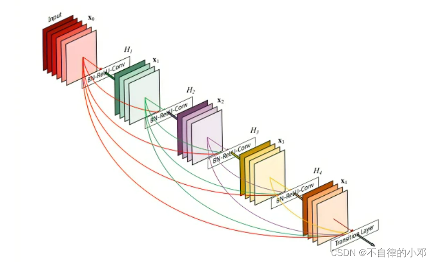

与ResNet是采用残差连接不同的是，DenseNet采用的是每一层都可以接收到前面所有层的输出，这样就可以获得前面所有层所提取的得到的特征，让信息更加丰富，提高信息复用，有助于提高模型的表达能力。显而易见的，DenseNet所用到的参数会更加多，计算也更复杂。

一般网络： $X_{l} = H_{1}(X_{l-1})$

ResNet: $X_{l} = H_{l}(X_{l-1}) + X_{l-1}$

DenseNet: $X_{l} = H_{l}([X_{1}+X_{2}+......+X_{l}])$

在DenseNet中有三个重要的组成部分growth_rate(增长率)，DenseBlock(稠密块)，TransitionLayer(过渡层)，接下来一一介绍这三个参数在DenseNet中的作用。

growth_rate:表示每个稠密块（dense block）中每一层输出的通道数或特征图的增长率。它定义了每个层对最终输出的贡献程度。

DenseBlock:由多个稠密层(DenseLayer)组成，稠密层的组成为：BN，ReLu，Conv(1×1)，BN，ReLu，Conv(3×3)。在稠密块中，每个层都直接连接到前面所有层的输出，形成稠密连接。稠密块内的层之间通过堆叠的方式连接在一起，这样可以使信息更加丰富，并促进特征的传递和重用。

TransitionLayer:过渡层的作用是为了控制模型的维度和特征图的尺寸，同时保持密集连接的特性。过渡层在两个稠密块之间，通常包含一个卷积一个池化。

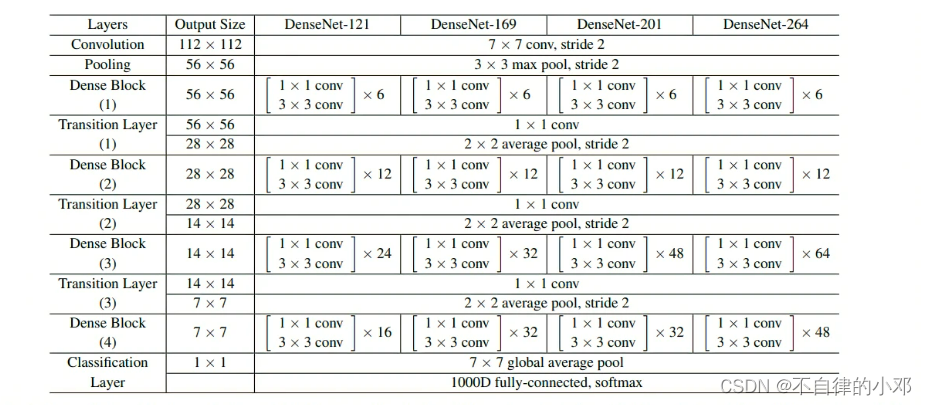
根据上图可以写出DenseNet。

①构建网络模型：

import torch.nn as nn import torch from torchvision import models class _DenseLayer(nn.Module): def __init__(self, num_input_features, growth_rate, bn_size, drop_rate=0): super(_DenseLayer, self).__init__() self.drop_rate = drop_rate self.dense_layer = nn.Sequential( nn.BatchNorm2d(num_input_features), nn.ReLU(inplace=True), nn.Conv2d(in_channels=num_input_features, out_channels=bn_size * growth_rate, kernel_size=1, stride=1, padding=0, bias=False), nn.BatchNorm2d(bn_size * growth_rate), nn.ReLU(inplace=True), nn.Conv2d(in_channels=bn_size * growth_rate, out_channels=growth_rate, kernel_size=3, stride=1, padding=1, bias=False) ) self.dropout = nn.Dropout(p=self.drop_rate) def forward(self, x): y = self.dense_layer(x) if self.drop_rate > 0: y = self.dropout(y) return torch.cat([x, y], dim=1) class _DenseBlock(nn.Module): def __init__(self, num_layers, num_input_features, bn_size, growth_rate, drop_rate=0): super(_DenseBlock, self).__init__() layers = [] for i in range(num_layers): layers.append(_DenseLayer(num_input_features + i * growth_rate, growth_rate, bn_size, drop_rate)) self.layers = nn.Sequential(*layers) def forward(self, x): return self.layers(x) class _TransitionLayer(nn.Module): def __init__(self, num_input_features, num_output_features): super(_TransitionLayer, self).__init__() self.transition_layer = nn.Sequential( nn.BatchNorm2d(num_input_features), nn.ReLU(inplace=True), nn.Conv2d(in_channels=num_input_features, out_channels=num_output_features, kernel_size=1, stride=1, padding=0, bias=False), nn.AvgPool2d(kernel_size=2, stride=2) ) def forward(self, x): return self.transition_layer(x) class DenseNet(nn.Module): def __init__(self, num_init_features=64, growth_rate=32, blocks=(6, 12, 24, 16), bn_size=4, drop_rate=0, num_classes=1000): super(DenseNet, self).__init__() self.features = nn.Sequential( nn.Conv2d(in_channels=3, out_channels=num_init_features, kernel_size=7, stride=2, padding=3, bias=False), nn.BatchNorm2d(num_init_features), nn.ReLU(inplace=True), nn.MaxPool2d(kernel_size=3, stride=2, padding=1) ) num_features = num_init_features self.layer1 = _DenseBlock(num_layers=blocks[0], num_input_features=num_features, growth_rate=growth_rate, bn_size=bn_size, drop_rate=drop_rate) num_features = num_features + blocks[0] * growth_rate self.transtion1 = _TransitionLayer(num_input_features=num_features, num_output_features=num_features // 2) num_features = num_features // 2 #向下取整除法 self.layer2 = _DenseBlock(num_layers=blocks[1], num_input_features=num_features, growth_rate=growth_rate, bn_size=bn_size, drop_rate=drop_rate) num_features = num_features + blocks[1] * growth_rate self.transtion2 = _TransitionLayer(num_input_features=num_features, num_output_features=num_features // 2) num_features = num_features // 2 self.layer3 = _DenseBlock(num_layers=blocks[2], num_input_features=num_features, growth_rate=growth_rate, bn_size=bn_size, drop_rate=drop_rate) num_features = num_features + blocks[2] * growth_rate self.transtion3 = _TransitionLayer(num_input_features=num_features, num_output_features=num_features // 2) num_features = num_features // 2 self.layer4 = _DenseBlock(num_layers=blocks[3], num_input_features=num_features, growth_rate=growth_rate, bn_size=bn_size, drop_rate=drop_rate) num_features = num_features + blocks[3] * growth_rate self.avgpool = nn.AdaptiveAvgPool2d((1, 1)) self.fc = nn.Linear(num_features, num_classes) def forward(self, x): x = self.features(x) x = self.layer1(x) x = self.transtion1(x) x = self.layer2(x) x = self.transtion2(x) x = self.layer3(x) x = self.transtion3(x) x = self.layer4(x) x = self.avgpool(x) x = torch.flatten(x, start_dim=1) x = self.fc(x) return x def DenseNet121(num_classes): return DenseNet(blocks=(6, 12, 24, 16), num_classes=num_classes) def DenseNet169(num_classes): return DenseNet(blocks=(6, 12, 32, 32), num_classes=num_classes) def DenseNet201(num_classes): return DenseNet(blocks=(6, 12, 48, 32), num_classes=num_classes) def DenseNet264(num_classes): return DenseNet(blocks=(6, 12, 64, 48), num_classes=num_classes) def read_densenet121(): device = torch.device('cuda' if torch.cuda.is_available() else 'cpu') model = models.densenet121(pretrained=True) model.to(device) print(model) def get_densenet121(flag, num_classes): if flag: net = models.densenet121(pretrained=True) num_input = net.classifier.in_features net.classifier = nn.Linear(num_input, num_classes) else: net = DenseNet121(num_classes) return net if __name__ == '__main__': test_set = torch.randn(64,3,32,32) Model = get_densenet121(flag=False,num_classes=10) output = Model(test_set) print(output.size())

②加载数据并训练网络：

讯享网import time from torchvision.transforms import Compose,Normalize,Resize,ToTensor from torchvision.datasets import CIFAR10 import torchvision.datasets from torch.utils.data import DataLoader from torchvision import transforms from DenseNet import * device = torch.device('cuda:3' if torch.cuda.is_available() else 'cpu') batch_size = 8 def CIFAR10_loader(size,train=True): transform_fn = Compose([ transforms.RandomHorizontalFlip(), transforms.RandomVerticalFlip(), transforms.RandomRotation([0, 180]), Resize((size,size)), ToTensor(), Normalize(mean=[0.485,0.456,0.406],std=[0.229,0.224,0.225]), ]) dataset = CIFAR10(root='../CIFAR10', train=train, transform=transform_fn, download=True) data_loader = DataLoader(dataset,batch_size=32,shuffle=True) return data_loader train_dataloader = CIFAR10_loader(size=32,train=True) test_dataloader = CIFAR10_loader(size=32,train=False) def evaluate_accuracy(data_iter, net, device=None): if device is None and isinstance(net, torch.nn.Module): device = list(net.parameters())[0].device acc_sum, n = 0.0, 0 with torch.no_grad(): for X, y in data_iter: net.eval() acc_sum += (net(X.to(device)).argmax(dim=1) == y.to(device)).float().sum().cpu().item() net.train() n += y.shape[0] return acc_sum / n def train(net, train_iter, test_iter, optimizer, device, num_epochs): net = net.to(device) print("training on ", device) loss = torch.nn.CrossEntropyLoss() for epoch in range(num_epochs): train_l_sum, train_acc_sum, n, batch_count, start = 0.0, 0.0, 0, 0, time.time() for X, y in train_iter: X = X.to(device) y = y.to(device) y_hat = net(X) l = loss(y_hat, y) optimizer.zero_grad() l.backward() optimizer.step() train_l_sum += l.cpu().item() train_acc_sum += (y_hat.argmax(dim=1) == y).sum().cpu().item() n += y.shape[0] batch_count += 1 test_acc = evaluate_accuracy(test_iter, net) print('epoch %d, loss %.4f, train acc %.3f%%, test acc %.3f%%, time %.1f sec' % (epoch + 1, train_l_sum / batch_count, 100*train_acc_sum / n, 100*test_acc, time.time() - start)) model = get_densenet121(flag=False, num_classes=10) num_epochs = 30 learning_rate = 0.001 optimizer = torch.optim.Adam(model.parameters(), lr=learning_rate) train(model, train_dataloader, test_dataloader, optimizer, device, num_epochs)

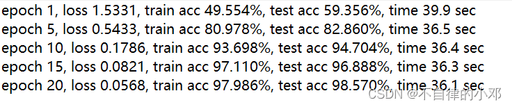
③训练结果：

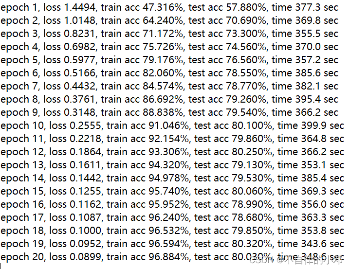
这个是在没有加入数据增强时的训练结果，和VGG，GoogleNet一样，发生了过拟合，都是因为模型太大，数据不足以支撑模型的训练。下面可以看一下，加入数据增强后的训练结果。

可以看出，loss上升，训练集和测试集的acc都下降了，这是因为过拟合使得模型对于未出现过的数据的泛化能力下降，所以导致了这种情况。虽然加入了数据增强，还是会过拟合，最大的原因还是，数据集虽然加入数据增强，但是数据还是太小，不适合用于大模型。

DenseNet采用的稠密连接，让参数的复用率大大提高，并且层与层之间的连接，使得梯度能够更好的传播，减轻了梯度消失的问题。

7.总结

LeNet，AlexNet，VGG，ResNet，GoogleNet，DenseNet都是卷积神经网络历程中的经典架构，每一个架构都在之前的架构上做出优化，并且在图像分类等任务上取得了显著的性能提升。当然不同的数据集，不同的要求，需要选择适合的模型去处理，不然很容易发生预期之外的情况(过拟合)。学习这些模型能够让初学者对于深度学习和卷积神经网络有更深入的了解。

总之，卷积神经网络是近几年计算机视觉领域中最重要的技术之一，学习不同的模型和技术，能够帮助技术人员应对不同场景，提高效率。

引言：

1.LeNet

2.AlexNet

3.VGG

4.GoogleNet

5.ResNet

6.DenseNet

7.总结

相关推荐