一.背景

Canny边缘检测算子是John F. Canny于1986年开发出来的一个多级边缘检测算法。它的目标是找到一个最优的边缘检测算法，最优边缘检测的含义是：①好的检测- 算法能够尽可能多地标识出图像中的实际边缘。②好的定位- 标识出的边缘要与实际图像中的实际边缘尽可能接近。③最小响应- 图像中的边缘只能标识一次，并且可能存在的图像噪声不应标识为边缘。

二.思路

1.Canny算子的基本步骤
①去噪，图像平滑。
任何边缘检测算法都不可能在未经处理的原始数据上很好地處理，一般采用的方法是利用原始数据与高斯核进行卷积，平滑处理。
②用一阶偏导的有限差分来计算梯度的幅值和方向。
计算一阶偏导用于找出灰度值变化较大的像素点，一般用Sobel算子。
③对梯度幅值进行非极大化抑制。
仅仅得到全局的梯度并不足以确定边缘，因此为确定边缘，必须保留局部梯度最大的点，而抑制非极大值。（non-maxima suppression,NMS）
解决方法：利用梯度的方向。
④边缘连接。
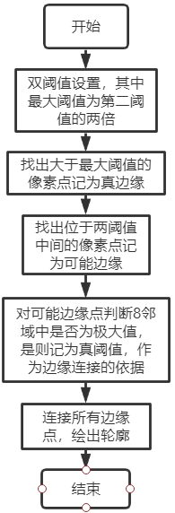
采用双阈值的方法进行边缘连接。

2.具体流程
对canny算子的四个步骤分别采用四个函数编写，最后利用主程序按顺序调用四个函数得到一个canny算子，并在每个过程中展示一次处理的结果，用于体现每个步骤的作用。
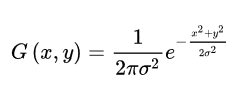
①图像平滑处理：
利用高斯滤波器对原始的图像，用高斯核函数：

讯享网
先对x方向进行卷积，再对y方向进行卷积，得到平滑处理后的图像。

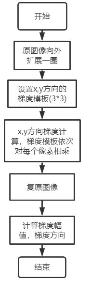
②Sobel边缘检测算子计算一阶偏导有限差分：
先将上一步的图像的上下左右各扩展一圈，为了能处理原始图像的边缘像素；然后设置Sobel算子的x和y方向的梯度模板，分别为：

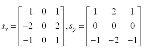
将图像的每个像素分别与xy模板进行相乘叠加，得到该像素点的x,y梯度值，再将扩展的图像复原。最后，每个像素的梯度幅值为：x,y方向的梯度值得平方和开根号得到，梯度方向为反正切值（y梯度/x梯度），将得到得值输出。

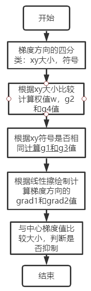
③梯度幅值的非极大值抑制
利用下图的线性插值原理计算在8邻域中中间像素点是否为极大值。

线性插值的公式为：

其中，w为根据梯度的角度决定的权重大小。
由梯度角度的大小得到梯度方向的四分类：y梯度是否大于x梯度，以及，y梯度与x梯度符号是否相同。
由y梯度与x梯度的大小比较：
当y大于x时得到权值的计算公式为：绝对值（x梯度/y梯度），g2=左方梯度值，g4=右方梯度值；且当y与x同号，g1=左上角梯度值，g3=右下角梯度值；当y与x不同号，g1=左下方梯度值，g3=右上方梯度值。
当y小于x时得到权值的计算公式为：绝对值（y梯度/x梯度），g2=上方梯度值，g4=下方梯度值；且当y与x同号，g1=左上角梯度值，g3=右下角梯度值；当y与x不同号，g1=左下方梯度值，g3=右上方梯度值。
最后根据计算得到的g1234和权值w计算梯度方向上的两个值，与中间值进行比较，看是否对中间值进行抑制。

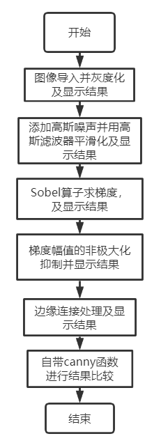
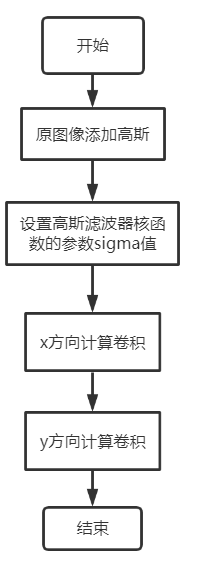
3.流程图
①主程序流程图为：

②高斯滤波平滑处理流程图为：

③Sobel算子流程图为：

④非极大值抑制的流程图为：

⑤边缘连接流程图为：

三.MATLAB代码

①主程序：cannytest.m

clear;clc; image=imread('Lena.jpg'); image=rgb2gray(image); %灰度化 %% 步骤一 添加高斯噪声并用高斯滤波平滑化 image_gaussnoise=imnoise(image,'gaussian',0,0.01); %添加高斯噪声 subplot(2,4,1); imshow(image_gaussnoise); title('添加高斯噪声'); image_guassfilter=gaussFilter(image_gaussnoise,2); %卷积核sigma值设为2，平滑效果较好，且不模糊 subplot(2,4,2); imshow(image_guassfilter); title('高斯滤波平滑处理'); %% 步骤二 求梯度 [grad,gradx,grady,angle]=Sobel_filter(image_guassfilter,3); subplot(2,4,3); imshow(gradx); title('x方向梯度'); subplot(2,4,4); imshow(grady); title('y方向梯度'); subplot(2,4,5); imshow(grad); title('梯度'); %% 步骤三 梯度幅值非极大化抑制 nmsgrad=nms(grad,angle,gradx,grady); subplot(2,4,6); imshow(nmsgrad); title('非极大值抑制后梯度'); %% 步骤四 双阈值算法检测和连接边缘 edgee=edge_correct(nmsgrad); subplot(2,4,7); imshow(edgee); title('边缘连接后的canny算子最终结果'); %% 用matlab自带的canny算子函数实现边缘检测作为结果的对比 ed = edge(image_gaussnoise,'canny', 0.5); subplot(2,4,8); imshow(ed); title('matlab自带的边缘检测函数'); 

②步骤一：高斯平滑:gaussFilter.m

讯享网%% 高斯平滑滤波函数（利用matlab自带的函数设计） function output=gaussFilter(image,sigma) output=image; ksize=double(uint8(3*sigma)*2+1);%窗口大小一半为3*sigma window = fspecial('gaussian', [1,ksize], sigma); %使用1行ksize列的高斯核对图像先进行x方向卷积，再进行y方向卷积 for i = 1:size(image,3) ret = imfilter(image(:,:,i),window,'replicate'); ret = imfilter(ret,window','replicate'); output(:,:,i) = ret; end end 

③步骤二：sobel算子求梯度：Sobel_filter.m

%% Sobel算子计算梯度得到边缘图像 function [output,outputx,outputy,outputangle]=Sobel_filter(image,n) image=double(image); [h,w]=size(image); %% 原灰度图像一圈扩展1个像素 big_image = zeros(h+2,w+2); for i = 2:h+1 for j = 2:w+1 big_image(i,j) = image(i-1,j-1); end end %% 设置Sobel算子x,y方向模板 Hx = [-1,-2,-1;0,0,0;1,2,1]; Hy = Hx'; %% x,y方向梯度计算 gradx_image = zeros(h+2,w+2); grady_image = zeros(h+2,w+2); W = zeros(n,n);%n阶的卷积核 for i = 1:h for j = 1:w %模板移动窗口 W = big_image(i:i+2,j:j+2); Sx = Hx .* W; Sy = Hy .* W; gradx_image(i+1,j+1) = sum(sum(Sx)); grady_image(i+1,j+1) = sum(sum(Sy)); end end %% 将一圈扩展1个像素的图像复原 gradx = zeros(h,w); grady = zeros(h,w); for i = 1:h for j = 1:w gradx(i,j) = gradx_image(i+1,j+1); grady(i,j) = grady_image(i+1,j+1); end end %sobel梯度 angle_grad=atand(grady./gradx); %求梯度方向(角度制） grad = sqrt(gradx.^2 + grady.^2); %得到图像的sobel梯度 outputx=uint8(gradx); outputy=uint8(grady); output=uint8(grad); outputangle=angle_grad; end 

④步骤三：非极大值抑制处理：nms.m

讯享网%% 梯度幅值非极大值抑制 function output=nms(grad,gradangle,gradx,grady) grad=double(grad); [h,w]=size(grad); %% 处理角度 sector=zeros(h,w); canny1=zeros(h,w); sector((gradangle>=45)&(gradangle<=-45))=0;%y方向梯度大于x梯度 sector((gradangle<45)&(gradangle>-45))=1;%y方向梯度小于x梯度 sector(gradangle>=0)=2;%x，y方向梯度符号相同 sector(gradangle<0)=3;%x，y方向梯度符号不同 %% 抑制算法实现，用线性插值算出梯度方向上的梯度值 weight=zeros(h,w); %权重初始化 grad1=zeros(h,w); %各值初始化 grad2=zeros(h,w); grad3=zeros(h,w); grad4=zeros(h,w); gradTemp1=zeros(h,w); gradTemp2=zeros(h,w); for i= 2:(h-1) for j = 2:(w-1) if grad(i,j)==0 %梯度为0，不是边缘点 sector(i,j)=0; else if 0 == sector(h,w) %y大于x weight(i,j)=abs(gradx(i,j))/abs(grady(i,j)); %权重的计算 grad2(i,j)=grad(i-1,j); grad4(i,j)=grad(i+1,j); if 2 == sector(h,w) grad1(i,j)=grad(i-1,j-1); grad3(i,j)=grad(i+1,j+1); elseif 3 == sector(h,w) grad1(i,j)=grad(i-1,j+1); grad3(i,j)=grad(i+1,j-1); end elseif 1 == sector(i,j) weight(i,j)=abs(grady(i,j))/abs(gradx(i,j)); grad2(i,j)=grad(i,j-1); grad4(i,j)=grad(i,j+1); if 2 == sector(h,w) grad1(i,j)=grad(i+1,j+1); grad3(i,j)=grad(i-1,j-1); elseif 3 == sector(h,w) grad1(i,j)=grad(i-1,j+1); grad3(i,j)=grad(i+1,j-1); end end gradTemp1(i,j) = weight(i,j) * grad1(i,j) + (1 - weight(i,j)) * grad2(i,j); %上方的梯度值 gradTemp2(i,j) = weight(i,j) * grad3(i,j) + (1 - weight(i,j)) * grad4(i,j); %下方的梯度值 if (grad(i,j) >= gradTemp1(i,j) && grad(i,j) >= gradTemp2(i,j)) canny1(i,j) = grad(i,j); %在邻域内为极大值，是边缘点 else canny1(i,j) = 0; end end end end output=uint8(canny1); 

⑤步骤四：边缘连接：edge_correct.m

%% 双阈值算法检测和连接边缘 function output=edge_correct(grad) grad=double(grad); [h,w]=size(grad); %定义双阈值：EP_MIN、EP_MAX，且EP_MAX = 2 * EP_MIN EP_MIN = 50; EP_MAX = EP_MIN * 2; EdgeLarge = zeros(h,w);%记录真边缘 EdgeBetween = zeros(h,w);%记录可能的边缘点 for i = 1:h for j = 1:w if grad(i,j) >= EP_MAX%小于小阈值，不可能为边缘点 EdgeLarge(i,j) = grad(i,j)+80; elseif grad(i,j) >= EP_MIN EdgeBetween(i,j) = grad(i,j); end end end %把EdgeLarge的边缘连成连续的轮廓 MAXSIZE = ; Queue = zeros(MAXSIZE,2);%用数组模拟队列 front = 1;%队头 rear = 1;%队尾 edge = zeros(h,w); for i = 1:h for j = 1:w if EdgeLarge(i,j) > 0 %强点入队 Queue(rear,1) = i; Queue(rear,2) = j; rear = rear + 1; edge(i,j) = EdgeLarge(i,j); EdgeLarge(i,j) = 0;%避免重复计算 end while front ~= rear%队不空 %队头出队 temp_i = Queue(front,1); temp_j = Queue(front,2); front = front + 1; %8-连通域寻找可能的边缘点 %左上方 if EdgeBetween(temp_i - 1,temp_j - 1) > 0 %把在强点周围的弱点变为强点 EdgeLarge(temp_i - 1,temp_j - 1) = grad(temp_i - 1,temp_j - 1); EdgeBetween(temp_i - 1,temp_j - 1) = 0;%避免重复计算 %入队 Queue(rear,1) = temp_i - 1; Queue(rear,2) = temp_j - 1; rear = rear + 1; end %正上方 if EdgeBetween(temp_i - 1,temp_j) > 0%把在强点周围的弱点变为强点 EdgeLarge(temp_i - 1,temp_j) = grad(temp_i - 1,temp_j); EdgeBetween(temp_i - 1,temp_j) = 0; %入队 Queue(rear,1) = temp_i - 1; Queue(rear,2) = temp_j; rear = rear + 1; end %右上方 if EdgeBetween(temp_i - 1,temp_j + 1) > 0%把在强点周围的弱点变为强点 EdgeLarge(temp_i - 1,temp_j + 1) = grad(temp_i - 1,temp_j + 1); EdgeBetween(temp_i - 1,temp_j + 1) = 0; %入队 Queue(rear,1) = temp_i - 1; Queue(rear,2) = temp_j + 1; rear = rear + 1; end %正左方 if EdgeBetween(temp_i,temp_j - 1) > 0%把在强点周围的弱点变为强点 EdgeLarge(temp_i,temp_j - 1) = grad(temp_i,temp_j - 1); EdgeBetween(temp_i,temp_j - 1) = 0; %入队 Queue(rear,1) = temp_i; Queue(rear,2) = temp_j - 1; rear = rear + 1; end %正右方 if EdgeBetween(temp_i,temp_j + 1) > 0%把在强点周围的弱点变为强点 EdgeLarge(temp_i,temp_j + 1) = grad(temp_i,temp_j + 1); EdgeBetween(temp_i,temp_j + 1) = 0; %入队 Queue(rear,1) = temp_i; Queue(rear,2) = temp_j + 1; rear = rear + 1; end %左下方 if EdgeBetween(temp_i + 1,temp_j - 1) > 0%把在强点周围的弱点变为强点 EdgeLarge(temp_i + 1,temp_j - 1) = grad(temp_i + 1,temp_j - 1); EdgeBetween(temp_i + 1,temp_j - 1) = 0; %入队 Queue(rear,1) = temp_i + 1; Queue(rear,2) = temp_j - 1; rear = rear + 1; end %正下方 if EdgeBetween(temp_i + 1,temp_j) > 0%把在强点周围的弱点变为强点 EdgeLarge(temp_i + 1,temp_j) = grad(temp_i + 1,temp_j); EdgeBetween(temp_i + 1,temp_j) = 0; %入队 Queue(rear,1) = temp_i + 1; Queue(rear,2) = temp_j; rear = rear + 1; end %右下方 if EdgeBetween(temp_i + 1,temp_j + 1) > 0%把在强点周围的弱点变为强点 EdgeLarge(temp_i + 1,temp_j + 1) = grad(temp_i + 1,temp_j + 1); EdgeBetween(temp_i + 1,temp_j + 1) = 0; %入队 Queue(rear,1) = temp_i + 1; Queue(rear,2) = temp_j + 1; rear = rear + 1; end end end end output=uint8(edge); end 

结果
共得到8张灰度图，对canny算子每个步骤的分析为：
①图二：高斯滤波平滑处理后图像能处理掉一部分噪声，使图像更加平滑，能避免后续处理描绘了噪声的边缘。
②图三为x方向梯度，图四为y方向梯度，图五为梯度幅值：
梯度计算后，轮廓已将基本描绘出，但不太清晰，且有些假轮廓；
③图六：非极大值抑制处理，能去掉假轮廓，仅保留真轮廓边缘。
④图七：边缘连接处理，并加深了轮廓颜色。
⑤图八：利用matlab自带的canny算子函数做边缘检测，作为对比。

四.python代码

1.主程序

讯享网# canny算子实现边缘检测 # 主程序 from __future__ import division from gaussian_filter import gaussian from gradient import gradient from nonmax_suppression import maximum from double_thresholding import thresholding import numpy as np import matplotlib.image as imgplt import matplotlib.pyplot as plt class tracking: def __init__(self, tr): self.im = tr[0] strongs = tr[1] self.vis = np.zeros(im.shape, bool) self.dx = [1, 0, -1, 0, -1, -1, 1, 1] self.dy = [0, 1, 0, -1, 1, -1, 1, -1] for s in strongs: if not self.vis[s]: self.dfs(s) for i in range(self.im.shape[0]): for j in range(self.im.shape[1]): self.im[i, j] = 1.0 if self.vis[i, j] else 0.0 def dfs(self, origin): q = [origin] while len(q) > 0: s = q.pop() self.vis[s] = True self.im[s] = 1 for k in range(len(self.dx)): for c in range(1, 16): nx, ny = s[0] + c * self.dx[k], s[1] + c * self.dy[k] if self.exists(nx, ny) and (self.im[nx, ny] >= 0.5) and (not self.vis[nx, ny]): q.append((nx, ny)) pass def exists(self, x, y): return x >= 0 and x < self.im.shape[0] and y >= 0 and y < self.im.shape[1] if __name__ == '__main__': im = imgplt.imread('Lena.jpg') plt.subplot(3, 2, 1) plt.imshow(im) plt.axis('off') plt.title('Original') im = im[:, :, 0] gim = gaussian(im) grim, gphase = gradient(gim) gmax = maximum(grim, gphase) thres = thresholding(gmax) edge = tracking(thres) plt.gray() plt.subplot(3, 2, 2) plt.imshow(gim) plt.axis('off') plt.title('Gaussian') plt.subplot(3, 2, 3) plt.imshow(grim) plt.axis('off') plt.title('Gradient') plt.subplot(3, 2, 4) plt.imshow(gmax) plt.axis('off') plt.title('Non-Maximum suppression') plt.subplot(3, 2, 5) plt.imshow(thres[0]) plt.axis('off') plt.title('Double thresholding') plt.subplot(3, 2, 6) plt.imshow(edge.im) plt.axis('off') plt.title('Edges') plt.show() 

2.步骤一：图像平滑

# canny算子步骤1：图像平滑 # 使用gauss函数实现：5*5 from __future__ import division import numpy as np import matplotlib.image as imgplt import matplotlib.pyplot as plt def gaussian(im): b = np.array([[2, 4, 5, 2, 2], [4, 9, 12, 9, 4], [5, 12, 15, 12, 5], [4, 9, 12, 9, 4], [2, 4, 5, 4, 2]]) / 156 kernel = np.zeros(im.shape) kernel[:b.shape[0], :b.shape[1]] = b fim = np.fft.fft2(im) fkernel = np.fft.fft2(kernel) fil_im = np.fft.ifft2(fim * fkernel) return abs(fil_im).astype(int) if __name__ == "__main__": im = imgplt.imread('Lena.jpg') im = im[:, :, 0] plt.gray() plt.subplot(1, 2, 1) plt.imshow(im) plt.axis('off') plt.title('Original') plt.subplot(1, 2, 2) plt.imshow(gaussian(im)) plt.axis('off') plt.title('Filtered') plt.show() 

3.步骤二：梯度计算

讯享网# canny算子步骤2：梯度计算 from __future__ import division from gaussian_filter import gaussian import numpy as np import matplotlib.image as imgplt import matplotlib.pyplot as plt def gradient(im): # Sobel operator op1 = np.array([[-1, 0, 1], [-2, 0, 2], [-1, 0, 1]]) op2 = np.array([[-1, -2, -1], [ 0, 0, 0], [ 1, 2, 1]]) kernel1 = np.zeros(im.shape) kernel1[:op1.shape[0], :op1.shape[1]] = op1 kernel1 = np.fft.fft2(kernel1) kernel2 = np.zeros(im.shape) kernel2[:op2.shape[0], :op2.shape[1]] = op2 kernel2 = np.fft.fft2(kernel2) fim = np.fft.fft2(im) Gx = np.real(np.fft.ifft2(kernel1 * fim)).astype(float) Gy = np.real(np.fft.ifft2(kernel2 * fim)).astype(float) G = np.sqrt(Gx2 + Gy2) Theta = np.arctan2(Gy, Gx) * 180 / np.pi return G, Theta if __name__ == '__main__': im = imgplt.imread('Lena.jpg') im = im[:, :, 0] gim = gaussian(im) grim, gphase = gradient(gim) plt.gray() plt.subplot(2, 2, 1) plt.imshow(im) plt.axis('off') plt.title('Original') plt.subplot(2, 2, 2) plt.imshow(gim) plt.axis('off') plt.title('Gaussian') plt.subplot(2, 2, 3) plt.imshow(grim) plt.axis('off') plt.title('Gradient') plt.show() 

4.步骤三：梯度幅值非极大值抑制

# canny算子步骤3：梯度幅值非极大值抑制 from __future__ import division from gaussian_filter import gaussian from gradient import gradient import numpy as np import matplotlib.image as imgplt import matplotlib.pyplot as plt def maximum(det, phase): gmax = np.zeros(det.shape) for i in range(gmax.shape[0]): for j in range(gmax.shape[1]): if phase[i][j] < 0: phase[i][j] += 360 if ((j + 1) < gmax.shape[1]) and ((j - 1) >= 0) and ((i + 1) < gmax.shape[0]) and ((i - 1) >= 0): # 0 degrees if (phase[i][j] >= 337.5 or phase[i][j] < 22.5) or (phase[i][j] >= 157.5 and phase[i][j] < 202.5): if det[i][j] >= det[i][j + 1] and det[i][j] >= det[i][j - 1]: gmax[i][j] = det[i][j] # 45 degrees if (phase[i][j] >= 22.5 and phase[i][j] < 67.5) or (phase[i][j] >= 202.5 and phase[i][j] < 247.5): if det[i][j] >= det[i - 1][j + 1] and det[i][j] >= det[i + 1][j - 1]: gmax[i][j] = det[i][j] # 90 degrees if (phase[i][j] >= 67.5 and phase[i][j] < 112.5) or (phase[i][j] >= 247.5 and phase[i][j] < 292.5): if det[i][j] >= det[i - 1][j] and det[i][j] >= det[i + 1][j]: gmax[i][j] = det[i][j] # 135 degrees if (phase[i][j] >= 112.5 and phase[i][j] < 157.5) or (phase[i][j] >= 292.5 and phase[i][j] < 337.5): if det[i][j] >= det[i - 1][j - 1] and det[i][j] >= det[i + 1][j + 1]: gmax[i][j] = det[i][j] return gmax if __name__ == '__main__': im = imgplt.imread('Lena.jpg') im = im[:, :, 0] gim = gaussian(im) grim, gphase = gradient(gim) gmax = maximum(grim, gphase) plt.gray() plt.subplot(2, 2, 1) plt.imshow(im) plt.axis('off') plt.title('Original') plt.subplot(2, 2, 2) plt.imshow(gim) plt.axis('off') plt.title('Gaussian') plt.subplot(2, 2, 3) plt.imshow(grim) plt.axis('off') plt.title('Gradient') plt.subplot(2, 2, 4) plt.imshow(gmax) plt.axis('off') plt.title('Non-Maximum suppression') plt.show() 

5.步骤四：边缘连接

讯享网# canny算子步骤4：边缘连接 # 边缘连接方法为使用双阈值 from __future__ import division from gaussian_filter import gaussian from gradient import gradient from nonmax_suppression import maximum import numpy as np import matplotlib.image as imgplt import matplotlib.pyplot as plt def thresholding(im): thres = np.zeros(im.shape) strong = 1.0 weak = 0.5 mmax = np.max(im) lo, hi = 0.1 * mmax, 0.8 * mmax strongs = [] for i in range(im.shape[0]): for j in range(im.shape[1]): px = im[i][j] if px >= hi: thres[i][j] = strong strongs.append((i, j)) elif px >= lo: thres[i][j] = weak return thres, strongs if __name__ == '__main__': im = imgplt.imread('Lena.jpg') im = im[:, :, 0] gim = gaussian(im) grim, gphase = gradient(gim) gmax = maximum(grim, gphase) thres = thresholding(gmax) plt.gray() plt.subplot(3, 2, 1) plt.imshow(im) plt.axis('off') plt.title('Original') plt.subplot(3, 2, 2) plt.imshow(gim) plt.axis('off') plt.title('Gaussian') plt.subplot(3, 2, 3) plt.imshow(grim) plt.axis('off') plt.title('Gradient') plt.subplot(3, 2, 4) plt.imshow(gmax) plt.axis('off') plt.title('Non-Maximum suppression') plt.subplot(3, 2, 5) plt.imshow(thres[0]) plt.axis('off') plt.title('Double thresholding') plt.show() 

结果