2025年特征工程主要包括哪些内容（特征工程主要包括哪些内容和方法）

大家好，我是讯享网，很高兴认识大家。
 <p style="margin-left:8px;text-align:right;"><span style="color:rgb(136,136,136);">来源：DeepHub IMBA</span></p><p style="margin-left:8px;text-align:right;"><span style="color:rgb(136,136,136);">作者：Muhammad Ihsan</span></p><hr /><p style="margin-left:8px;">在数据分析和机器学习领域，从原始数据中提取有价值的信息是一个关键步骤。这个过程不仅有助于辅助决策，还能预测未来趋势。为了实现这一目标，特征工程技术显得尤为重要。</p><p>特征工程是将原始数据转化为更具信息量的特征的过程。本文将详细介绍十种基础特征工程技术，包括其基本原理和实现示例。首先，我们需要导入必要的库以确保代码的正常运行。以下是本文中使用的主要库：</p><p> </p><p style="margin-left:8px;"> <span style="color:rgb(119,0,136);">import</span> <span style="color:rgb(0,0,0);">pandas</span> <span style="color:rgb(119,0,136);">as</span> <span style="color:rgb(0,0,0);">pd</span>  <span style="color:rgb(170,85,0);"># 用于数据处理和操作</span><br /> <span style="color:rgb(119,0,136);">import</span> <span style="color:rgb(0,0,0);">numpy</span> <span style="color:rgb(119,0,136);">as</span> <span style="color:rgb(0,0,0);">np</span>  <span style="color:rgb(170,85,0);"># 用于数值计算</span><br /> <span style="color:rgb(119,0,136);">import</span> <span style="color:rgb(0,0,0);">matplotlib</span>.<span style="color:rgb(0,0,0);">pyplot</span> <span style="color:rgb(119,0,136);">as</span> <span style="color:rgb(0,0,0);">plt</span>  <span style="color:rgb(170,85,0);"># 用于数据可视化</span><br /> <span style="color:rgb(119,0,136);">import</span> <span style="color:rgb(0,0,0);">gensim</span>.<span style="color:rgb(0,0,0);">downloader</span> <span style="color:rgb(119,0,136);">as</span> <span style="color:rgb(0,0,0);">api</span>  <span style="color:rgb(170,85,0);"># 用于下载gensim提供的语料库</span><br /> <span style="color:rgb(119,0,136);">from</span> <span style="color:rgb(0,0,0);">gensim</span>.<span style="color:rgb(0,0,0);">models</span> <span style="color:rgb(119,0,136);">import</span> <span style="color:rgb(0,0,0);">Word2Vec</span>  <span style="color:rgb(170,85,0);"># 用于词嵌入</span><br /> <span style="color:rgb(119,0,136);">from</span> <span style="color:rgb(0,0,0);">sklearn</span>.<span style="color:rgb(0,0,0);">pipeline</span> <span style="color:rgb(119,0,136);">import</span> <span style="color:rgb(0,0,0);">Pipeline</span>  <span style="color:rgb(170,85,0);"># 用于构建数据处理管道</span><br /> <span style="color:rgb(119,0,136);">from</span> <span style="color:rgb(0,0,0);">sklearn</span>.<span style="color:rgb(0,0,0);">decomposition</span> <span style="color:rgb(119,0,136);">import</span> <span style="color:rgb(0,0,0);">PCA</span>  <span style="color:rgb(170,85,0);"># 用于主成分分析</span><br /> <span style="color:rgb(119,0,136);">from</span> <span style="color:rgb(0,0,0);">sklearn</span>.<span style="color:rgb(0,0,0);">datasets</span> <span style="color:rgb(119,0,136);">import</span> <span style="color:rgb(0,0,0);">load_iris</span>  <span style="color:rgb(170,85,0);"># 用于加载iris数据集</span><br /> <span style="color:rgb(119,0,136);">from</span> <span style="color:rgb(0,0,0);">sklearn</span>.<span style="color:rgb(0,0,0);">impute</span> <span style="color:rgb(119,0,136);">import</span> <span style="color:rgb(0,0,0);">SimpleImputer</span>  <span style="color:rgb(170,85,0);"># 用于数据插补</span><br /> <span style="color:rgb(119,0,136);">from</span> <span style="color:rgb(0,0,0);">sklearn</span>.<span style="color:rgb(0,0,0);">compose</span> <span style="color:rgb(119,0,136);">import</span> <span style="color:rgb(0,0,0);">ColumnTransformer</span>  <span style="color:rgb(170,85,0);"># 用于对数据集应用转换</span><br /> <br /> <span style="color:rgb(119,0,136);">from</span> <span style="color:rgb(0,0,0);">sklearn</span>.<span style="color:rgb(0,0,0);">feature_extraction</span>.<span style="color:rgb(0,0,0);">text</span> <span style="color:rgb(119,0,136);">import</span> <span style="color:rgb(0,0,0);">TfidfVectorizer</span>  <span style="color:rgb(170,85,0);"># 用于TF-IDF实现</span><br /> <span style="color:rgb(119,0,136);">from</span> <span style="color:rgb(0,0,0);">sklearn</span>.<span style="color:rgb(0,0,0);">preprocessing</span> <span style="color:rgb(119,0,136);">import</span> <span style="color:rgb(0,0,0);">MinMaxScaler</span>, <span style="color:rgb(0,0,0);">StandardScaler</span>  <span style="color:rgb(170,85,0);"># 用于数据缩放</span></p><hr /><p style="margin-left:8px;"><strong>1、数据插补</strong></p><p style="margin-left:8px;">数据插补是处理缺失数据的重要技术，它通过用其他值替换缺失数据来完善数据集。在实际应用中，许多算法（如线性回归和逻辑回归）无法直接处理包含缺失值的数据集。因此我们通常有两种选择：</p><p style="margin-left:8px;">删除包含缺失值的行或列</p><p style="margin-left:8px;">对缺失值进行插补</p><p style="margin-left:8px;">数据插补的方法多样，包括：</p><p style="margin-left:8px;">使用常数值填充（如0、1、2等）</p><p style="margin-left:8px;">使用统计量填充（如均值或中位数）</p><p style="margin-left:8px;">使用相邻数据值填充（如前值或后值）</p><p style="margin-left:8px;">构建预测模型估计缺失值</p><p style="margin-left:8px;">以下是一个数据插补的实现示例：</p><p style="margin-left:8px;"> <span style="color:rgb(0,0,0);">data</span> <span style="color:rgb(152,26,26);">=</span> <span style="color:rgb(0,0,0);">pd</span>.<span style="color:rgb(0,0,0);">DataFrame</span>({<br />     <span style="color:rgb(34,162,201);">'doors'</span>: [<span style="color:rgb(17,102,68);">2</span>, <span style="color:rgb(0,0,0);">np</span>.<span style="color:rgb(0,0,0);">nan</span>, <span style="color:rgb(17,102,68);">2</span>, <span style="color:rgb(0,0,0);">np</span>.<span style="color:rgb(0,0,0);">nan</span>, <span style="color:rgb(17,102,68);">4</span>],<br />     <span style="color:rgb(34,162,201);">'topspeed'</span>: [<span style="color:rgb(17,102,68);">100</span>, <span style="color:rgb(0,0,0);">np</span>.<span style="color:rgb(0,0,0);">nan</span>, <span style="color:rgb(17,102,68);">150</span>, <span style="color:rgb(17,102,68);">200</span>, <span style="color:rgb(0,0,0);">np</span>.<span style="color:rgb(0,0,0);">nan</span>],<br />     <span style="color:rgb(34,162,201);">'model'</span>: [<span style="color:rgb(34,162,201);">'Daihatsu'</span>, <span style="color:rgb(34,162,201);">'Toyota'</span>, <span style="color:rgb(34,162,201);">'Suzuki'</span>, <span style="color:rgb(34,162,201);">'BYD'</span>,<span style="color:rgb(34,162,201);">'Wuling'</span>]<br /> })<br /> <br /> <span style="color:rgb(0,0,0);">doors_imputer</span> <span style="color:rgb(152,26,26);">=</span> <span style="color:rgb(0,0,0);">Pipeline</span>(<span style="color:rgb(0,0,0);">steps</span><span style="color:rgb(152,26,26);">=</span>[<br />     (<span style="color:rgb(34,162,201);">'imputer'</span>, <span style="color:rgb(0,0,0);">SimpleImputer</span>(<span style="color:rgb(0,0,0);">strategy</span><span style="color:rgb(152,26,26);">=</span><span style="color:rgb(34,162,201);">'constant'</span>, <span style="color:rgb(0,0,0);">fill_value</span><span style="color:rgb(152,26,26);">=</span><span style="color:rgb(17,102,68);">4</span>))<br /> ])<br /> <br /> <span style="color:rgb(0,0,0);">topspeed_imputer</span> <span style="color:rgb(152,26,26);">=</span> <span style="color:rgb(0,0,0);">Pipeline</span>(<span style="color:rgb(0,0,0);">steps</span><span style="color:rgb(152,26,26);">=</span>[<br />     (<span style="color:rgb(34,162,201);">'imputer'</span>, <span style="color:rgb(0,0,0);">SimpleImputer</span>(<span style="color:rgb(0,0,0);">strategy</span><span style="color:rgb(152,26,26);">=</span><span style="color:rgb(34,162,201);">'median'</span>))<br /> ])<br /> <br /> <span style="color:rgb(0,0,0);">pipeline</span> <span style="color:rgb(152,26,26);">=</span> <span style="color:rgb(0,0,0);">ColumnTransformer</span>(<br />     <span style="color:rgb(0,0,0);">transformers</span><span style="color:rgb(152,26,26);">=</span>[<br />         (<span style="color:rgb(34,162,201);">'doors_imputer'</span>, <span style="color:rgb(0,0,0);">doors_imputer</span>, [<span style="color:rgb(34,162,201);">'doors'</span>]),<br />         (<span style="color:rgb(34,162,201);">'topspeed_imputer'</span>, <span style="color:rgb(0,0,0);">topspeed_imputer</span>, [<span style="color:rgb(34,162,201);">'topspeed'</span>])<br />     ],<br />     <span style="color:rgb(0,0,0);">remainder</span><span style="color:rgb(152,26,26);">=</span><span style="color:rgb(34,162,201);">'passthrough'</span><br /> )<br /> <br /> <span style="color:rgb(0,0,0);">transformed</span> <span style="color:rgb(152,26,26);">=</span> <span style="color:rgb(0,0,0);">pipeline</span>.<span style="color:rgb(0,0,0);">fit_transform</span>(<span style="color:rgb(0,0,0);">data</span>)<br /> <br /> <span style="color:rgb(0,0,0);">transformed_df</span> <span style="color:rgb(152,26,26);">=</span> <span style="color:rgb(0,0,0);">pd</span>.<span style="color:rgb(0,0,0);">DataFrame</span>(<span style="color:rgb(0,0,0);">transformed</span>, <span style="color:rgb(0,0,0);">columns</span><span style="color:rgb(152,26,26);">=</span>[<span style="color:rgb(34,162,201);">'doors'</span>, <span style="color:rgb(34,162,201);">'topspeed'</span>, <span style="color:rgb(34,162,201);">'model'</span>])</p><p style="margin-left:8px;">在这个例子中创建了一个包含汽车数据的DataFrame，其中doors和topspeed列存在缺失值。对于doors列，使用常数4进行填充（假设大多数汽车有4个门）。对于topspeed列，使用中位数进行填充。</p><p style="margin-left:8px;">下图展示了插补前后的数据对比：</p><p style="margin-left:8px;text-align:center;"><img src='https://file1.elecfans.com//web2/M00/0A/A4/wKgZomckTr2APXwiAABaGfc-FNE383.jpg' alt='数据分析' /></p><p>可以观察到doors列的缺失值被填充为4，而topspeed列的缺失值被填充为数据的中位数。</p><hr /><p>数据分箱是将连续变量转换为离散分类变量的技术。这种技术在日常生活中常被无意识地使用，例如将人按年龄段分类。数据分箱的主要目的包括：</p><ol><li>简化数据，将连续值转换为离散类别</li><li>处理非线性关系</li></ol><p style="margin-left:8px;">减少数据中的噪声和异常值</p><p>以下是一个数据分箱的实现示例：</p><p style="margin-left:8px;"> <span style="color:rgb(0,0,0);">np</span>.<span style="color:rgb(0,0,0);">random</span>.<span style="color:rgb(0,0,0);">seed</span>(<span style="color:rgb(17,102,68);">42</span>)<br /> <span style="color:rgb(0,0,0);">data</span> <span style="color:rgb(152,26,26);">=</span> <span style="color:rgb(0,0,0);">pd</span>.<span style="color:rgb(0,0,0);">DataFrame</span>({<span style="color:rgb(34,162,201);">'age'</span> : <span style="color:rgb(0,0,0);">np</span>.<span style="color:rgb(0,0,0);">random</span>.<span style="color:rgb(0,0,0);">randint</span>(<span style="color:rgb(17,102,68);">0</span>, <span style="color:rgb(17,102,68);">100</span>, <span style="color:rgb(17,102,68);">100</span>)})<br /> <span style="color:rgb(0,0,0);">data</span>[<span style="color:rgb(34,162,201);">'category'</span>] <span style="color:rgb(152,26,26);">=</span> <span style="color:rgb(0,0,0);">pd</span>.<span style="color:rgb(0,0,0);">cut</span>(<span style="color:rgb(0,0,0);">data</span>[<span style="color:rgb(34,162,201);">'age'</span>], [<span style="color:rgb(17,102,68);">0</span>, <span style="color:rgb(17,102,68);">2</span>, <span style="color:rgb(17,102,68);">11</span>, <span style="color:rgb(17,102,68);">18</span>, <span style="color:rgb(17,102,68);">65</span>, <span style="color:rgb(17,102,68);">101</span>], <span style="color:rgb(0,0,0);">labels</span><span style="color:rgb(152,26,26);">=</span>[<span style="color:rgb(34,162,201);">'infants'</span>, <span style="color:rgb(34,162,201);">'children'</span>, <span style="color:rgb(34,162,201);">'teenagers'</span>, <span style="color:rgb(34,162,201);">'adults'</span>, <span style="color:rgb(34,162,201);">'elders'</span>])<br /> <span style="color:rgb(51,0,170);">print</span>(<span style="color:rgb(0,0,0);">data</span>)<br /> <span style="color:rgb(51,0,170);">print</span>(<span style="color:rgb(0,0,0);">data</span>[<span style="color:rgb(34,162,201);">'category'</span>].<span style="color:rgb(0,0,0);">value_counts</span>())<br /> <span style="color:rgb(0,0,0);">data</span>[<span style="color:rgb(34,162,201);">'category'</span>].<span style="color:rgb(0,0,0);">value_counts</span>().<span style="color:rgb(0,0,0);">plot</span>(<span style="color:rgb(0,0,0);">kind</span><span style="color:rgb(152,26,26);">=</span><span style="color:rgb(34,162,201);">'bar'</span>)</p><p>在这个例子中，我们生成了100个0到100之间的随机整数作为年龄数据，然后将其分为五个类别：婴儿、儿童、青少年、成年人和老年人。以下是分箱结果的可视化：</p><p style="margin-left:8px;text-align:center;"><img src='https://file1.elecfans.com//web2/M00/0A/A4/wKgZomckTr2AFwK4AABGSU_0NkI441.jpg' alt='数据分析' /></p><p>通过数据分箱，可以更直观地理解数据的分布情况。在某些算法中，经过分箱处理的离散数据可能比原始的连续数据更有优势。</p><hr /><p style="margin-left:8px;">对数变换是将特征值从x转换为log(x)的技术。这种方法常用于处理高度偏斜的数据分布或存在大量异常值的情况。</p><p style="margin-left:8px;">对数变换在线性回归和逻辑回归等模型中特别有用，因为它可以将乘法关系转换为加法关系，从而简化模型。</p><p>以下是对数变换的实现示例：</p><p style="margin-left:8px;"> <span style="color:rgb(0,0,0);">rskew_data</span> <span style="color:rgb(152,26,26);">=</span> <span style="color:rgb(0,0,0);">np</span>.<span style="color:rgb(0,0,0);">random</span>.<span style="color:rgb(0,0,0);">exponential</span>(<span style="color:rgb(0,0,0);">scale</span><span style="color:rgb(152,26,26);">=</span><span style="color:rgb(17,102,68);">2</span>, <span style="color:rgb(0,0,0);">size</span><span style="color:rgb(152,26,26);">=</span><span style="color:rgb(17,102,68);">100</span>)<br /> <br /> <span style="color:rgb(0,0,0);">log_data</span> <span style="color:rgb(152,26,26);">=</span> <span style="color:rgb(0,0,0);">np</span>.<span style="color:rgb(0,0,0);">log</span>(<span style="color:rgb(0,0,0);">rskew_data</span>)<br /> <br /> <span style="color:rgb(0,0,0);">plt</span>.<span style="color:rgb(0,0,0);">title</span>(<span style="color:rgb(34,162,201);">'Right Skewed Data'</span>)<br /> <span style="color:rgb(0,0,0);">plt</span>.<span style="color:rgb(0,0,0);">hist</span>(<span style="color:rgb(0,0,0);">rskew_data</span>, <span style="color:rgb(0,0,0);">bins</span><span style="color:rgb(152,26,26);">=</span><span style="color:rgb(17,102,68);">10</span>)<br /> <span style="color:rgb(0,0,0);">plt</span>.<span style="color:rgb(0,0,0);">show</span>()<br /> <span style="color:rgb(0,0,0);">plt</span>.<span style="color:rgb(0,0,0);">title</span>(<span style="color:rgb(34,162,201);">'Log Transformed Data'</span>)<br /> <span style="color:rgb(0,0,0);">plt</span>.<span style="color:rgb(0,0,0);">hist</span>(<span style="color:rgb(0,0,0);">log_data</span>, <span style="color:rgb(0,0,0);">bins</span><span style="color:rgb(152,26,26);">=</span><span style="color:rgb(17,102,68);">20</span>)<br /> <span style="color:rgb(0,0,0);">plt</span>.<span style="color:rgb(0,0,0);">show</span>()</p><p>在这个例子中，生成了100个右偏的数据点，然后对其进行对数变换。下图展示了变换前后的数据分布对比：<img src='https://file1.elecfans.com//web2/M00/0A/A4/wKgZomckTr2AHqYCAAA6E4zsVCc406.jpg' alt='数据分析' /></p><p style="margin-left:8px;">需要注意的是，对数变换并不会自动将数据分布变为正态分布，它主要用于减少数据的偏度。</p><hr /><p>数据缩放是将数据调整到特定范围或满足特定条件的预处理技术。常见的缩放方法包括：</p><ul><li><strong>最小-最大缩放：</strong>将数据调整到[0, 1]区间</li><li><strong>标准化：</strong>将数据调整为均值为0，标准差为1的分布</li></ul><p>最小-最大缩放主要用于将数据归一化到特定范围，而标准化则考虑了数据的分布特征。以下是数据缩放的实现示例：</p><p> <span style="color:rgb(0,0,0);">data</span> <span style="color:rgb(152,26,26);">=</span> <span style="color:rgb(0,0,0);">np</span>.<span style="color:rgb(0,0,0);">array</span>([<span style="color:rgb(17,102,68);">1</span>, <span style="color:rgb(17,102,68);">2</span>, <span style="color:rgb(17,102,68);">3</span>, <span style="color:rgb(17,102,68);">4</span>, <span style="color:rgb(17,102,68);">5</span>, <span style="color:rgb(17,102,68);">6</span>, <span style="color:rgb(17,102,68);">7</span>, <span style="color:rgb(17,102,68);">8</span>, <span style="color:rgb(17,102,68);">9</span>, <span style="color:rgb(17,102,68);">10</span>]).<span style="color:rgb(0,0,0);">reshape</span>(<span style="color:rgb(152,26,26);">-</span><span style="color:rgb(17,102,68);">1</span>, <span style="color:rgb(17,102,68);">1</span>)<br /> <br /> <span style="color:rgb(0,0,0);">scaler</span> <span style="color:rgb(152,26,26);">=</span> <span style="color:rgb(0,0,0);">MinMaxScaler</span>()<br /> <span style="color:rgb(0,0,0);">minmax</span> <span style="color:rgb(152,26,26);">=</span> <span style="color:rgb(0,0,0);">scaler</span>.<span style="color:rgb(0,0,0);">fit_transform</span>(<span style="color:rgb(0,0,0);">data</span>)<br /> <br /> <span style="color:rgb(0,0,0);">scaler</span> <span style="color:rgb(152,26,26);">=</span> <span style="color:rgb(0,0,0);">StandardScaler</span>()<br /> <span style="color:rgb(0,0,0);">standard</span> <span style="color:rgb(152,26,26);">=</span> <span style="color:rgb(0,0,0);">scaler</span>.<span style="color:rgb(0,0,0);">fit_transform</span>(<span style="color:rgb(0,0,0);">data</span>)<br /> <br /> <span style="color:rgb(0,0,0);">df</span> <span style="color:rgb(152,26,26);">=</span> <span style="color:rgb(0,0,0);">pd</span>.<span style="color:rgb(0,0,0);">DataFrame</span>({<span style="color:rgb(34,162,201);">'original'</span>:<span style="color:rgb(0,0,0);">data</span>.<span style="color:rgb(0,0,0);">flatten</span>(),<span style="color:rgb(34,162,201);">'Min-Max Scaling'</span>:<span style="color:rgb(0,0,0);">minmax</span>.<span style="color:rgb(0,0,0);">flatten</span>(),<span style="color:rgb(34,162,201);">'Standard Scaling'</span>:<span style="color:rgb(0,0,0);">standard</span>.<span style="color:rgb(0,0,0);">flatten</span>()})<br /> <span style="color:rgb(0,0,0);">df</span></p><p style="margin-left:8px;">下图展示了原始数据、最小-最大缩放后的数据和标准化后的数据的对比：</p><p style="text-align:center;"><img src='https://file1.elecfans.com//web2/M00/0A/A4/wKgZomckTr2AD2yGAAB5Mf0pIxA762.jpg' alt='数据分析' /></p><p>可以观察到，最小-最大缩放将数据调整到[0, 1]区间，而标准化后的数据均值接近0，标准差接近1。</p><hr /><p style="margin-left:8px;">One-Hot编码是处理分类数据的常用方法，特别适用于那些没有固有顺序的名义变量。这种技术将每个分类变量转换为一系列二进制特征。</p><p style="margin-left:8px;">One-Hot编码的工作原理如下：</p><ol><li>对于分类特征中的每个唯一值，创建一个新的二进制列。</li></ol><p style="margin-left:8px;">在新创建的列中，如果原始数据中出现了相应的分类值，则标记为1，否则为0。</p><p style="margin-left:8px;">这种方法也被称为虚拟编码（dummy encoding）。</p><p>以下是One-Hot编码的实现示例：</p><p style="margin-left:8px;"> <span style="color:rgb(0,0,0);">data</span> <span style="color:rgb(152,26,26);">=</span> <span style="color:rgb(0,0,0);">pd</span>.<span style="color:rgb(0,0,0);">DataFrame</span>({<span style="color:rgb(34,162,201);">'models'</span>:[<span style="color:rgb(34,162,201);">'toyota'</span>,<span style="color:rgb(34,162,201);">'ferrari'</span>,<span style="color:rgb(34,162,201);">'byd'</span>,<span style="color:rgb(34,162,201);">'lamborghini'</span>,<span style="color:rgb(34,162,201);">'honda'</span>,<span style="color:rgb(34,162,201);">'tesla'</span>],<br />                     <span style="color:rgb(34,162,201);">'speed'</span>:[<span style="color:rgb(34,162,201);">'slow'</span>,<span style="color:rgb(34,162,201);">'fast'</span>,<span style="color:rgb(34,162,201);">'medium'</span>,<span style="color:rgb(34,162,201);">'fast'</span>,<span style="color:rgb(34,162,201);">'slow'</span>,<span style="color:rgb(34,162,201);">'medium'</span>]})<br /> <span style="color:rgb(0,0,0);">data</span> <span style="color:rgb(152,26,26);">=</span> <span style="color:rgb(0,0,0);">pd</span>.<span style="color:rgb(0,0,0);">concat</span>([<span style="color:rgb(0,0,0);">data</span>, <span style="color:rgb(0,0,0);">pd</span>.<span style="color:rgb(0,0,0);">get_dummies</span>(<span style="color:rgb(0,0,0);">data</span>[<span style="color:rgb(34,162,201);">'speed'</span>], <span style="color:rgb(0,0,0);">prefix</span><span style="color:rgb(152,26,26);">=</span><span style="color:rgb(34,162,201);">'speed'</span>)],<span style="color:rgb(0,0,0);">axis</span><span style="color:rgb(152,26,26);">=</span><span style="color:rgb(17,102,68);">1</span>)<br /> <span style="color:rgb(0,0,0);">data</span></p><p style="margin-left:8px;">下图展示了编码后的结果：</p><p><img src='https://file1.elecfans.com//web2/M00/0A/A4/wKgZomckTr2AeZBIAABlMcVqzN4949.jpg' alt='数据分析' /></p><p style="margin-left:8px;">'speed'列被转换为三个新的二进制列：'speed_fast'、'speed_medium'和'speed_slow'。每行在这些新列中只有一个1，其余为0，对应原始的速度类别。</p><p>当分类变量的唯一值数量很大时，One-Hot编码可能会导致特征空间的急剧膨胀。在这种情况下，可能需要考虑其他编码方法或降维技术。</p><hr /><p>目标编码是一种利用目标变量来编码分类特征的方法。这种技术特别适用于高基数的分类变量（即具有大量唯一值的变量）。目标编码的基本步骤如下：</p><ol style="list-style-type:decimal;"><li>对于分类特征中的每个类别，计算对应的目标变量统计量（如均值）。</li><li>用计算得到的统计量替换原始的类别值。</li></ol><p style="margin-left:8px;">以下是目标编码的一个简单实现：</p><p style="margin-left:8px;"> <span style="color:rgb(0,0,0);">fruits</span> <span style="color:rgb(152,26,26);">=</span> [<span style="color:rgb(34,162,201);">'banana'</span>,<span style="color:rgb(34,162,201);">'apple'</span>,<span style="color:rgb(34,162,201);">'durian'</span>,<span style="color:rgb(34,162,201);">'durian'</span>,<span style="color:rgb(34,162,201);">'apple'</span>,<span style="color:rgb(34,162,201);">'banana'</span>]<br /> <span style="color:rgb(0,0,0);">price</span> <span style="color:rgb(152,26,26);">=</span> [<span style="color:rgb(17,102,68);">120</span>,<span style="color:rgb(17,102,68);">100</span>,<span style="color:rgb(17,102,68);">110</span>,<span style="color:rgb(17,102,68);">150</span>,<span style="color:rgb(17,102,68);">140</span>,<span style="color:rgb(17,102,68);">160</span>]<br /> <span style="color:rgb(0,0,0);">data</span> <span style="color:rgb(152,26,26);">=</span> <span style="color:rgb(0,0,0);">pd</span>.<span style="color:rgb(0,0,0);">DataFrame</span>({<br />   <span style="color:rgb(34,162,201);">'fruit'</span>: <span style="color:rgb(0,0,0);">fruits</span>,<br />   <span style="color:rgb(34,162,201);">'price'</span>: <span style="color:rgb(0,0,0);">price</span><br /> })<br /> <span style="color:rgb(0,0,0);">data</span>[<span style="color:rgb(34,162,201);">'encoded_fruits'</span>] <span style="color:rgb(152,26,26);">=</span> <span style="color:rgb(0,0,0);">data</span>.<span style="color:rgb(0,0,0);">groupby</span>(<span style="color:rgb(34,162,201);">'fruit'</span>)[<span style="color:rgb(34,162,201);">'price'</span>].<span style="color:rgb(0,0,0);">transform</span>(<span style="color:rgb(34,162,201);">'mean'</span>)<br /> <span style="color:rgb(0,0,0);">data</span></p><p style="margin-left:8px;">结果如下图所示：</p><p style="text-align:center;"><img src='https://file1.elecfans.com//web2/M00/0A/A4/wKgZomckTr2AdxZgAAA8J6ovwM4071.jpg' alt='数据分析' /></p><p>我们用每种水果的平均价格替换了原始的水果名称。这种方法不仅可以处理高基数的分类变量，还能捕捉类别与目标变量之间的关系。使用目标编码时需要注意以下几点：</p><ol style="list-style-type:decimal;"><li>可能导致数据泄露，特别是在不做适当的交叉验证的情况下。</li><li>对异常值敏感，可能需要进行额外的异常值处理。</li><li>在测试集中遇到训练集中未出现的类别时，需要有合适的处理策略。</li></ol><hr /><p style="margin-left:8px;">主成分分析（Principal Component Analysis，PCA）是一种常用的无监督学习方法，主要用于降维和特征提取。PCA通过线性变换将原始特征投影到一个新的特征空间，使得新的特征（主成分）按方差大小排序。</p><p style="margin-left:8px;">PCA的主要步骤包括：</p><p style="margin-left:8px;">数据标准化</p><p style="margin-left:8px;">计算协方差矩阵</p><p style="margin-left:8px;">计算协方差矩阵的特征值和特征向量</p><p style="margin-left:8px;">选择主成分</p><p style="margin-left:8px;">投影数据到新的特征空间</p><p style="margin-left:8px;">以下是使用PCA的一个示例，我们使用著名的Iris数据集：</p><p style="margin-left:8px;"> <span style="color:rgb(0,0,0);">iris_data</span> <span style="color:rgb(152,26,26);">=</span> <span style="color:rgb(0,0,0);">load_iris</span>()<br /> <span style="color:rgb(0,0,0);">features</span> <span style="color:rgb(152,26,26);">=</span> <span style="color:rgb(0,0,0);">iris_data</span>.<span style="color:rgb(0,0,0);">data</span><br /> <span style="color:rgb(0,0,0);">targets</span> <span style="color:rgb(152,26,26);">=</span> <span style="color:rgb(0,0,0);">iris_data</span>.<span style="color:rgb(0,0,0);">target</span><br /> <br /> <span style="color:rgb(0,0,0);">features</span>.<span style="color:rgb(0,0,0);">shape</span><br /> <span style="color:rgb(170,85,0);"># 输出: (150, 4)</span><br /> <br /> <span style="color:rgb(0,0,0);">pca</span> <span style="color:rgb(152,26,26);">=</span> <span style="color:rgb(0,0,0);">PCA</span>(<span style="color:rgb(0,0,0);">n_components</span><span style="color:rgb(152,26,26);">=</span><span style="color:rgb(17,102,68);">2</span>)<br /> <span style="color:rgb(0,0,0);">pca_features</span> <span style="color:rgb(152,26,26);">=</span> <span style="color:rgb(0,0,0);">pca</span>.<span style="color:rgb(0,0,0);">fit_transform</span>(<span style="color:rgb(0,0,0);">features</span>)<br /> <br /> <span style="color:rgb(0,0,0);">pca_features</span>.<span style="color:rgb(0,0,0);">shape</span><br /> <span style="color:rgb(170,85,0);"># 输出: (150, 2)</span><br /> <br /> <span style="color:rgb(119,0,136);">for</span> <span style="color:rgb(0,0,0);">point</span> <span style="color:rgb(119,0,136);">in</span> <span style="color:rgb(51,0,170);">set</span>(<span style="color:rgb(0,0,0);">targets</span>):<br />     <span style="color:rgb(0,0,0);">plt</span>.<span style="color:rgb(0,0,0);">scatter</span>(<span style="color:rgb(0,0,0);">pca_features</span>[<span style="color:rgb(0,0,0);">targets</span> <span style="color:rgb(152,26,26);">==</span> <span style="color:rgb(0,0,0);">point</span>, <span style="color:rgb(17,102,68);">0</span>], <span style="color:rgb(0,0,0);">pca_features</span>[<span style="color:rgb(0,0,0);">targets</span> <span style="color:rgb(152,26,26);">==</span> <span style="color:rgb(0,0,0);">point</span>,<span style="color:rgb(17,102,68);">1</span>], <span style="color:rgb(0,0,0);">label</span><span style="color:rgb(152,26,26);">=</span><span style="color:rgb(0,0,0);">iris_data</span>.<span style="color:rgb(0,0,0);">target_names</span>[<span style="color:rgb(0,0,0);">point</span>])<br /> <span style="color:rgb(0,0,0);">plt</span>.<span style="color:rgb(0,0,0);">xlabel</span>(<span style="color:rgb(34,162,201);">'PCA Component 1'</span>)<br /> <span style="color:rgb(0,0,0);">plt</span>.<span style="color:rgb(0,0,0);">ylabel</span>(<span style="color:rgb(34,162,201);">'PCA Component 2'</span>)<br /> <span style="color:rgb(0,0,0);">plt</span>.<span style="color:rgb(0,0,0);">title</span>(<span style="color:rgb(34,162,201);">'PCA on Iris Dataset'</span>)<br /> <span style="color:rgb(0,0,0);">plt</span>.<span style="color:rgb(0,0,0);">legend</span>()<br /> <span style="color:rgb(0,0,0);">plt</span>.<span style="color:rgb(0,0,0);">show</span>()</p><p>结果如下图所示：<img src='https://file1.elecfans.com//web2/M00/0A/A4/wKgZomckTr2Ad7-eAAB2NrPNziw407.jpg' alt='数据分析' /></p><p style="margin-left:8px;">在这个例子中将原始的4维特征空间降至2维。从图中可以看出，即使在降维后，不同类别的数据点仍然保持了良好的可分性。</p><p style="margin-left:8px;">PCA的优点包括：</p><p style="margin-left:8px;">减少数据的维度，降低计算复杂度。</p><p style="margin-left:8px;">去除噪声和冗余信息。</p><p style="margin-left:8px;">有助于数据可视化。</p><p style="margin-left:8px;">PCA也有一些局限性：</p><p style="margin-left:8px;">可能导致一定程度的信息损失。</p><p style="margin-left:8px;">转换后的特征难以解释，因为每个主成分都是原始特征的线性组合。</p><ol><li>仅捕捉线性关系，对于非线性关系效果可能不佳。</li></ol><hr /><p style="margin-left:8px;">特征聚合是一种通过组合现有特征来创建新特征的方法。这种技术常用于时间序列数据、分组数据或者需要综合多个特征信息的场景。</p><p style="margin-left:8px;">常见的特征聚合方法包括：</p><p style="margin-left:8px;">统计聚合：如平均值、中位数、最大值、最小值等。</p><p style="margin-left:8px;">时间聚合：如按天、周、月等时间单位聚合数据。</p><p style="margin-left:8px;">分组聚合：根据某些类别特征对数据进行分组，然后在每个组内进行聚合。</p><p style="margin-left:8px;">以下是一个特征聚合的示例：</p><p style="margin-left:8px;"> <span style="color:rgb(0,0,0);">quarter</span> <span style="color:rgb(152,26,26);">=</span> [<span style="color:rgb(34,162,201);">'Q1'</span>,<span style="color:rgb(34,162,201);">'Q2'</span>,<span style="color:rgb(34,162,201);">'Q3'</span>,<span style="color:rgb(34,162,201);">'Q4'</span>]<br /> <span style="color:rgb(0,0,0);">car_sales</span> <span style="color:rgb(152,26,26);">=</span> [<span style="color:rgb(17,102,68);">10000</span>,<span style="color:rgb(17,102,68);">9850</span>,<span style="color:rgb(17,102,68);">13000</span>,<span style="color:rgb(17,102,68);">20000</span>]<br /> <span style="color:rgb(0,0,0);">motorbike_sales</span> <span style="color:rgb(152,26,26);">=</span> [<span style="color:rgb(17,102,68);">14000</span>,<span style="color:rgb(17,102,68);">18000</span>,<span style="color:rgb(17,102,68);">9000</span>,<span style="color:rgb(17,102,68);">11000</span>]<br /> <span style="color:rgb(0,0,0);">sparepart_sales</span> <span style="color:rgb(152,26,26);">=</span> [<span style="color:rgb(17,102,68);">5000</span>, <span style="color:rgb(17,102,68);">7000</span>,<span style="color:rgb(17,102,68);">3000</span>, <span style="color:rgb(17,102,68);">10000</span>]<br /> <br /> <span style="color:rgb(0,0,0);">data</span> <span style="color:rgb(152,26,26);">=</span> <span style="color:rgb(0,0,0);">pd</span>.<span style="color:rgb(0,0,0);">DataFrame</span>({<span style="color:rgb(34,162,201);">'car'</span>:<span style="color:rgb(0,0,0);">car_sales</span>,<br />     <span style="color:rgb(34,162,201);">'motorbike'</span>:<span style="color:rgb(0,0,0);">motorbike_sales</span>,<br />     <span style="color:rgb(34,162,201);">'sparepart'</span>:<span style="color:rgb(0,0,0);">sparepart_sales</span>}, <span style="color:rgb(0,0,0);">index</span><span style="color:rgb(152,26,26);">=</span><span style="color:rgb(0,0,0);">quarter</span>)<br /> <br /> <span style="color:rgb(0,0,0);">data</span>[<span style="color:rgb(34,162,201);">'avg_sales'</span>] <span style="color:rgb(152,26,26);">=</span> <span style="color:rgb(0,0,0);">data</span>[[<span style="color:rgb(34,162,201);">'car'</span>,<span style="color:rgb(34,162,201);">'motorbike'</span>,<span style="color:rgb(34,162,201);">'sparepart'</span>]].<span style="color:rgb(0,0,0);">mean</span>(<span style="color:rgb(0,0,0);">axis</span><span style="color:rgb(152,26,26);">=</span><span style="color:rgb(17,102,68);">1</span>).<span style="color:rgb(0,0,0);">astype</span>(<span style="color:rgb(51,0,170);">int</span>)<br /> <span style="color:rgb(0,0,0);">data</span>[<span style="color:rgb(34,162,201);">'total_sales'</span>] <span style="color:rgb(152,26,26);">=</span> <span style="color:rgb(0,0,0);">data</span>[[<span style="color:rgb(34,162,201);">'car'</span>,<span style="color:rgb(34,162,201);">'motorbike'</span>,<span style="color:rgb(34,162,201);">'sparepart'</span>]].<span style="color:rgb(0,0,0);">sum</span>(<span style="color:rgb(0,0,0);">axis</span><span style="color:rgb(152,26,26);">=</span><span style="color:rgb(17,102,68);">1</span>).<span style="color:rgb(0,0,0);">astype</span>(<span style="color:rgb(51,0,170);">int</span>)<br /> <br /> <span style="color:rgb(0,0,0);">data</span></p><p style="margin-left:8px;">结果如下图所示：</p><p><img src='https://file1.elecfans.com//web2/M00/0A/A4/wKgZomckTr6ALUKtAABZig7f2v0311.jpg' alt='数据分析' /></p><p style="margin-left:8px;">在这个例子中创建了两个新的特征：</p><p style="margin-left:8px;">'avg_sales'：每个季度不同产品的平均销售额。</p><p style="margin-left:8px;">'total_sales'：每个季度所有产品的总销售额。</p><p>这种聚合可以帮助我们从不同角度理解数据，发现可能被单个特征忽略的模式。</p><p style="margin-left:8px;">特征聚合的优点包括：</p><p style="margin-left:8px;">可以捕捉多个特征之间的关系。</p><p style="margin-left:8px;">减少特征的数量，有助于模型的解释和计算效率。</p><ol><li>可能创造出更有预测力的特征。</li></ol><p style="margin-left:8px;">在使用特征聚合时也需要注意：</p><p style="margin-left:8px;">聚合可能会导致一些细节信息的丢失。</p><p style="margin-left:8px;">需要领域知识来决定哪些聚合是有意义的。</p><ol><li>过度聚合可能会导致过拟合。</li></ol><hr /><p style="margin-left:8px;">TF-IDF（Term Frequency-Inverse Document Frequency）是一种广泛用于文本分析和信息检索的特征提取技术。它结合了词频（TF）和逆文档频率（IDF）两个指标，用于评估一个词对于一个文档集或一个语料库中的某一个文档的重要程度。</p><p style="margin-left:8px;">TF-IDF的计算基于以下两个概念：</p><p style="margin-left:8px;">词频（TF）：衡量一个词在文档中出现的频率。计算公式为：TF(t,d) = (词t在文档d中出现的次数) / (文档d中的总词数)</p><ol><li>逆文档频率（IDF）：衡量一个词在整个文档集中的普遍重要性。计算公式为：IDF(t) = log(总文档数 / 包含词t的文档数)</li></ol><p style="margin-left:8px;">TF-IDF的最终得分是TF和IDF的乘积：TF-IDF(t,d) = TF(t,d) * IDF(t)</p><p style="margin-left:8px;">以下是使用TF-IDF的一个示例：</p><p style="margin-left:8px;"> <span style="color:rgb(0,0,0);">texts</span> <span style="color:rgb(152,26,26);">=</span> [<span style="color:rgb(34,162,201);">"I eat rice with eggs."</span>,<br />         <span style="color:rgb(34,162,201);">"I also love to eat fried rice. Rice is the most delicious food in the world"</span>]<br /> <br /> <span style="color:rgb(0,0,0);">vectorizer</span> <span style="color:rgb(152,26,26);">=</span> <span style="color:rgb(0,0,0);">TfidfVectorizer</span>()<br /> <span style="color:rgb(0,0,0);">tfidfmatrix</span> <span style="color:rgb(152,26,26);">=</span> <span style="color:rgb(0,0,0);">vectorizer</span>.<span style="color:rgb(0,0,0);">fit_transform</span>(<span style="color:rgb(0,0,0);">texts</span>)<br /> <span style="color:rgb(0,0,0);">features</span> <span style="color:rgb(152,26,26);">=</span> <span style="color:rgb(0,0,0);">vectorizer</span>.<span style="color:rgb(0,0,0);">get_feature_names_out</span>()<br /> <span style="color:rgb(0,0,0);">data</span> <span style="color:rgb(152,26,26);">=</span> <span style="color:rgb(0,0,0);">pd</span>.<span style="color:rgb(0,0,0);">DataFrame</span>(<span style="color:rgb(0,0,0);">tfidfmatrix</span>.<span style="color:rgb(0,0,0);">toarray</span>(), <span style="color:rgb(0,0,0);">columns</span><span style="color:rgb(152,26,26);">=</span><span style="color:rgb(0,0,0);">features</span>)<br /> <br /> <span style="color:rgb(51,0,170);">print</span>(<span style="color:rgb(34,162,201);">"TF-IDF matrix"</span>)<br /> <span style="color:rgb(0,0,0);">data</span></p><p style="margin-left:8px;">结果如下图所示：</p><p style="margin-left:8px;text-align:center;"><img src='https://file1.elecfans.com//web2/M00/0A/A4/wKgZomckTr6ACdY4AAA1anYX_Ns905.jpg' alt='数据分析' /></p><p style="margin-left:8px;">在这个例子中：</p><p style="margin-left:8px;">第一行代表句子 "I eat rice with eggs."</p><ul><li>第二行代表句子 "I also love to eat fried rice. Rice is the most delicious food in the world"</li></ul><p>可以观察到，"rice" 这个词在第一个句子中的TF-IDF值（0.409）比在第二个句子中的值（0.349）更高。这是因为虽然 "rice" 在第二个句子中出现得更频繁，但第一个句子更短，使得 "rice" 在其中的相对重要性更高。</p><p style="margin-left:8px;">TF-IDF的主要优点包括：</p><p style="margin-left:8px;">能够反映词语在文档中的重要程度。</p><p style="margin-left:8px;">可以过滤掉常见词语，突出关键词。</p><ol><li>计算简单，易于理解和实现。</li></ol><p style="margin-left:8px;">TF-IDF也有一些局限性：</p><p style="margin-left:8px;">没有考虑词序和语法结构。</p><p style="margin-left:8px;">对于极短文本可能效果不佳。</p><ol><li>不能捕捉词语之间的语义关系。</li></ol><hr /><p style="margin-left:8px;">文本嵌入是将文本数据（如单词、短语或文档）映射到连续向量空间的技术。这种技术能够捕捉词语之间的语义关系，是现代自然语言处理中的基础技术之一。</p><p style="margin-left:8px;">常见的文本嵌入方法包括：</p><p style="margin-left:8px;">Word2Vec</p><p style="margin-left:8px;">GloVe (Global Vectors for Word Representation)</p><p style="margin-left:8px;">FastText</p><ol><li>BERT (Bidirectional Encoder Representations from Transformers)</li></ol><p style="margin-left:8px;">以下是使用Word2Vec进行文本嵌入的示例：</p><p> <span style="color:rgb(0,0,0);">corpus</span> <span style="color:rgb(152,26,26);">=</span> <span style="color:rgb(0,0,0);">api</span>.<span style="color:rgb(0,0,0);">load</span>(<span style="color:rgb(34,162,201);">'text8'</span>)  <br /> <span style="color:rgb(0,0,0);">model</span> <span style="color:rgb(152,26,26);">=</span> <span style="color:rgb(0,0,0);">Word2Vec</span>(<span style="color:rgb(0,0,0);">corpus</span>)  <br /> <span style="color:rgb(0,0,0);">dog</span> <span style="color:rgb(152,26,26);">=</span> <span style="color:rgb(0,0,0);">model</span>.<span style="color:rgb(0,0,0);">wv</span>[<span style="color:rgb(34,162,201);">'dog'</span>]<br /> <span style="color:rgb(51,0,170);">print</span>(<span style="color:rgb(34,162,201);">"Embedding vector for 'dog':
讯享网
“, dog)
输出结果示例：
数据分析
讯享网
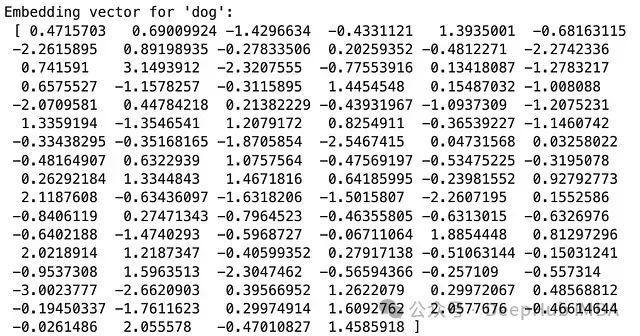
我们使用了gensim库提供的text8语料库（包含维基百科文本的前100,000,000个字节）来训练Word2Vec模型。每个词被映射到一个100维的向量空间中。
文本嵌入的一个重要特性是能够捕捉词语之间的语义关系。我们可以通过计算词向量之间的相似度来展示这一点：
cat = model.wv[‘cat’]
car = model.wv[‘car’]

dogvscat = model.wv.similarity(‘dog’,‘cat’)
dogvscar = model.wv.similarity(‘dog’,‘car’)

print(“Similarity:”)
print(“Dog vs Cat: “, dogvscat)
print(“Dog vs Car: “, dogvscar)
输出结果：
数据分析
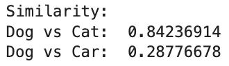
从结果可以看出，”dog”和”cat”的相似度明显高于”dog”和”car”的相似度，这符合我们的语义直觉。
文本嵌入的主要优点包括：
能够捕捉词语之间的语义关系。
可以处理高维稀疏的文本数据，将其转换为低维稠密的向量表示。
通过迁移学习，可以在小规模数据集上也能获得良好的表现。
文本嵌入也存在一些挑战：
训练高质量的嵌入模型通常需要大量的文本数据和计算资源。
词语的多义性可能无法被单一的静态向量完全捕捉。
对于特定领域的任务，可能需要在领域特定的语料上重新训练或微调嵌入模型。
本文介绍了十种基本的特征工程技术，涵盖了数值型、分类型和文本型数据的处理方法。每种技术都有其特定的应用场景和优缺点。在实际应用中，选择合适的特征工程技术需要考虑数据的特性、问题的性质以及模型的要求。often需要结合多种技术来获得**的特征表示。还有许多其他高级的特征工程技术未在本文中涉及，如时间序列特征工程、图像特征提取等。随着机器学习和深度学习技术的发展，特征工程的重要性可能会有所变化，但理解和掌握这些基本技术仍然是数据科学实践中的重要基础。
特征工程不仅是一门技术，更是一门艺术。它需要领域知识、直觉和经验的结合。通过不断的实践和实验，我们可以逐步提高特征工程的技能，从而为后续的机器学习任务奠定坚实的基础。
2025年特征工程主要包括哪些内容（特征工程主要包括哪些内容和方法）

相关推荐
