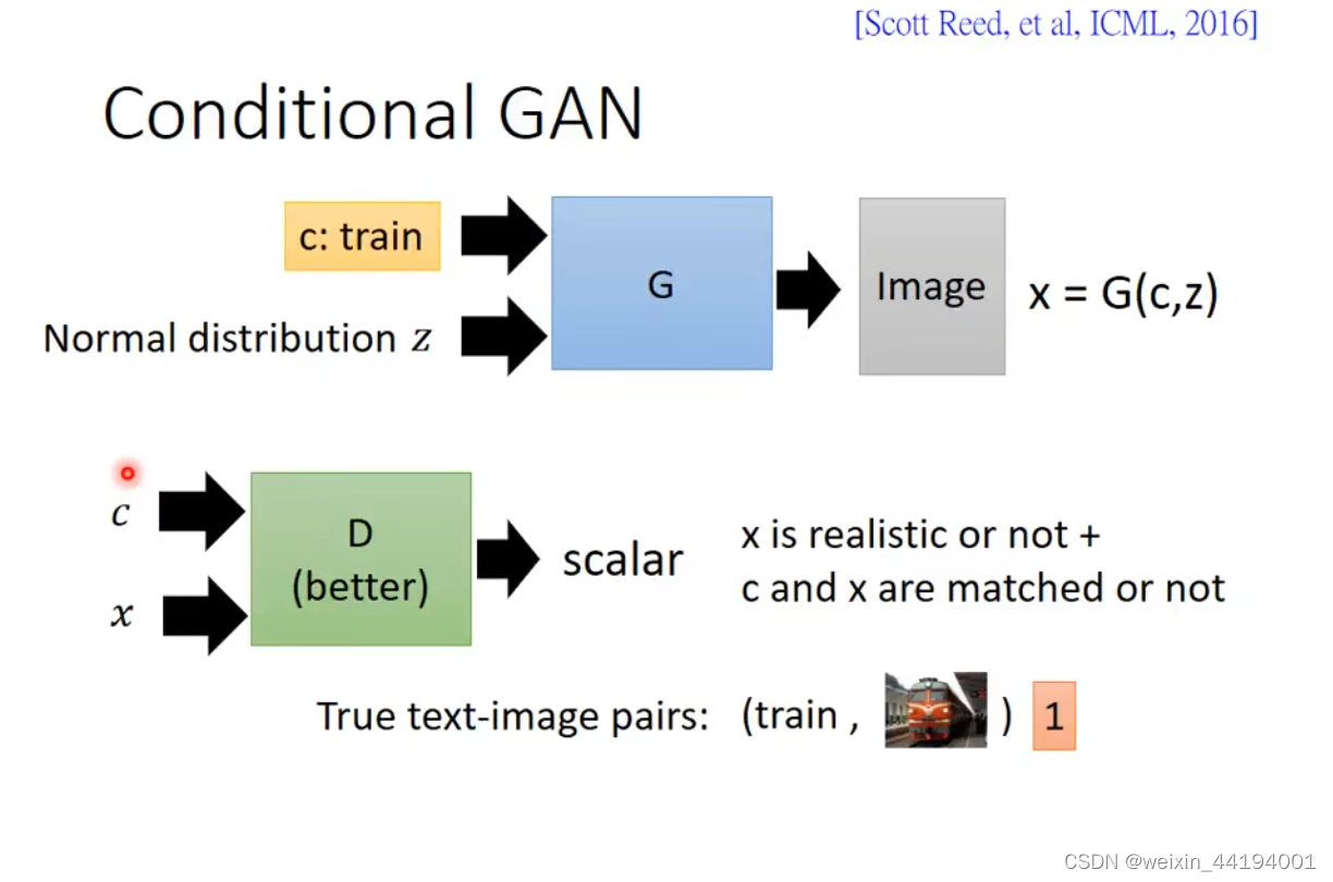
1.CGAN原理

生成器生成的图片被判别器认为是真实图片，那么标签就是1
其实判别器模型输出的是生成器生成的图片被判别器认为是真实图片的概率，再与标签1做交叉熵运算，进而反向传播训练生成器模型，调整参数，使得生成器生成的图片被判别器认为是真实图片的概率越来越大。

讯享网

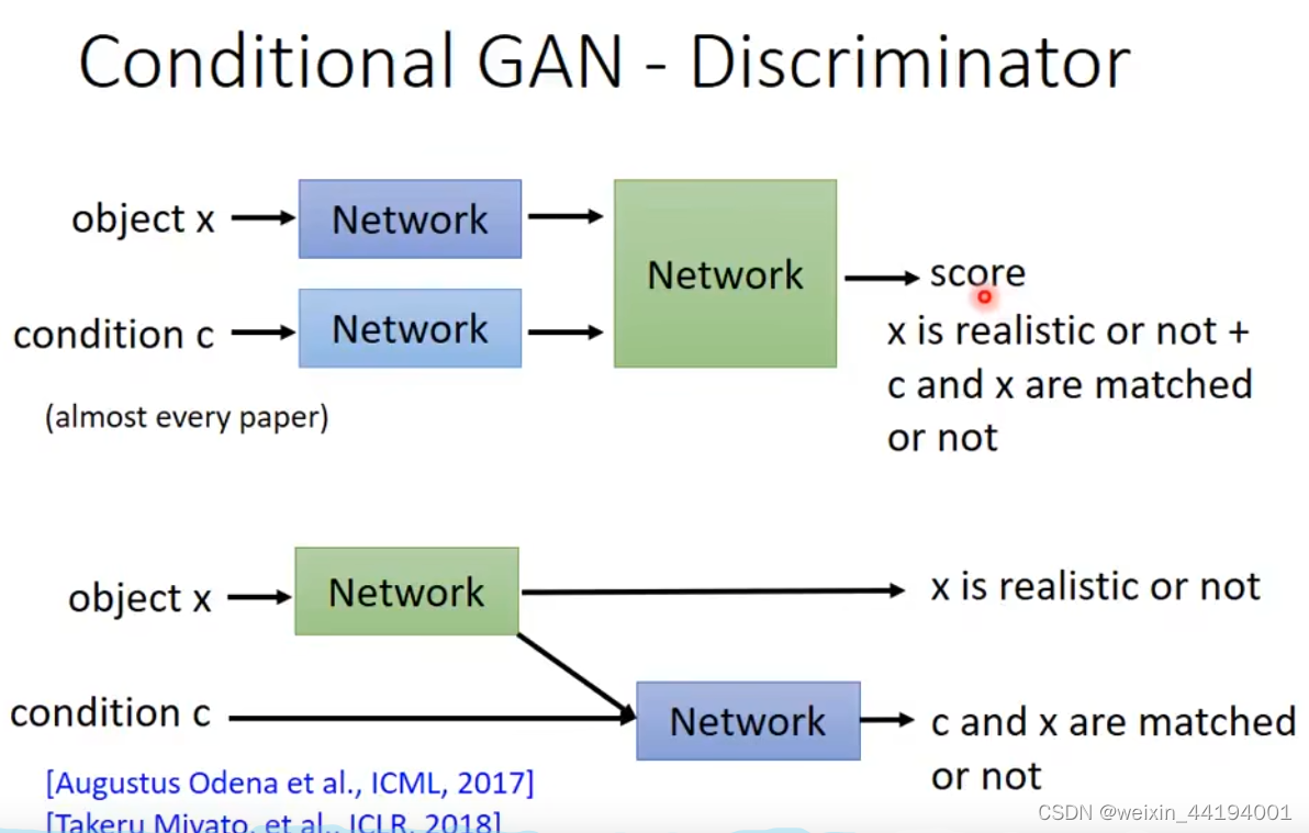
判别器的输入是
1.生成器输出的虚假图片x;
2.对应图片的标签c

来自真实数据集，且标签是对的，就是1
如果是生成器生成的虚假照片就直接是0，都不需要看是否与标签对应

上面第二张图的意思就是，当图片是来自真实数据集，再来看是否与标签对应

2.CGAN损失函数

上面这个值，生成器越小越好，即判别器认为真实图片是真实图片的概率越低越好，认为虚假图片是真实图片的概率越高越好
判别器越大越好，即判别器认为真实图片是真实图片的概率越大越好，认为虚假图片是真实图片的概率越小越好

criterion(output, label)

在判别器中，
1）output是预测来自真实数据集的图片和标签是否是真实且符合标签的概率，label是1
2）output是预测虚假图片是否是虚假图片的概率，label是0
在生成器中，
output是判别器预测虚假图片是否是真实图片的概率，label是1
以上三种，都是交叉熵越小越好

3.生成器和判别器的源码

class Generator(nn.Module): def __init__(self, num_channel=1, nz=100, nc=10, ngf=64): super(Generator, self).__init__() self.main = nn.Sequential( # 输入维度 110 x 1 x 1 nn.ConvTranspose2d(nz + nc, ngf * 8, 4, 1, 0, bias=False), nn.BatchNorm2d(ngf * 8), nn.ReLU(True), # 特征维度 (ngf*8) x 4 x 4 nn.ConvTranspose2d(ngf * 8, ngf * 4, 4, 2, 1, bias=False), nn.BatchNorm2d(ngf * 4), nn.ReLU(True), # 特征维度 (ngf*4) x 8 x 8 nn.ConvTranspose2d(ngf * 4, ngf * 2, 4, 2, 1, bias=False), nn.BatchNorm2d(ngf * 2), nn.ReLU(True), # 特征维度 (ngf*2) x 16 x 16 nn.ConvTranspose2d(ngf * 2, ngf, 4, 2, 1, bias=False), nn.BatchNorm2d(ngf), nn.ReLU(True), # 特征维度 (ngf) x 32 x 32 nn.ConvTranspose2d(ngf, num_channel, 4, 2, 1, bias=False), nn.Tanh() # 特征维度. (num_channel) x 64 x 64 ) self.apply(weights_init) def forward(self, input_z, onehot_label): input_ = torch.cat((input_z, onehot_label), dim=1) n, c = input_.size() input_ = input_.view(n, c, 1, 1) return self.main(input_) class Discriminator(nn.Module): def __init__(self, num_channel=1, nc=10, ndf=64): super(Discriminator, self).__init__() self.main = nn.Sequential( # 输入维度 (num_c3 # channel+nc) x 64 x 64 1*64*64的图像和10维的类别 10维类别先转换成10*64*64 然后合并就是11*64*64 # 输入通道 输出通道 卷积核的大小 步长 填充 #原始输入张量：b 11 64 64 nn.Conv2d(num_channel + nc, ndf, 4, 2, 1, bias=False), #b 64 32 32 nn.LeakyReLU(0.2, inplace=True), # 特征维度 (ndf) x 32 x 32 nn.Conv2d(ndf, ndf * 2, 4, 2, 1, bias=False), #b 64*2 16 16 nn.BatchNorm2d(ndf * 2), nn.LeakyReLU(0.2, inplace=True), # 特征维度 (ndf*2) x 16 x 16 nn.Conv2d(ndf * 2, ndf * 4, 4, 2, 1, bias=False), #b 64*4 8 8 nn.BatchNorm2d(ndf * 4), nn.LeakyReLU(0.2, inplace=True), # 特征维度 (ndf*4) x 8 x 8 nn.Conv2d(ndf * 4, ndf * 8, 4, 2, 1, bias=False), #b 64*8 4 4 nn.BatchNorm2d(ndf * 8), nn.LeakyReLU(0.2, inplace=True), # 特征维度 (ndf*8) x 4 x 4 nn.Conv2d(ndf * 8, 1, 4, 1, 0, bias=False), #b 1 1 1 其实就是一个数值，区间在正无穷到负无穷之间 nn.Sigmoid() ) self.apply(weights_init) def forward(self, images, onehot_label): device = 'cuda' if torch.cuda.is_available() else 'cpu' h, w = images.shape[2:] n, nc = onehot_label.shape[:2] label = onehot_label.view(n, nc, 1, 1) * torch.ones([n, nc, h, w]).to(device) input_ = torch.cat([images, label], 1) return self.main(input_) 

4.训练过程

讯享网 MODEL_G_PATH = "./" LOG_G_PATH = "Log_G.txt" LOG_D_PATH = "Log_D.txt" IMAGE_SIZE = 64 BATCH_SIZE = 128 WORKER = 1 LR = 0.0002 NZ = 100 NUM_CLASS = 10 EPOCH = 10 data_loader = loadMNIST(img_size=IMAGE_SIZE, batch_size=BATCH_SIZE) #原始图片宽高是28*28的，给改变成64*64 device = torch.device("cuda:0" if torch.cuda.is_available() else "cpu") netG = Generator().to(device) netD = Discriminator().to(device) criterion = nn.BCELoss() real_label = 1. fake_label = 0. optimizerD = optim.Adam(netD.parameters(), lr=LR, betas=(0.5, 0.999)) optimizerG = optim.Adam(netG.parameters(), lr=LR, betas=(0.5, 0.999)) g_writer = LossWriter(save_path=LOG_G_PATH) d_writer = LossWriter(save_path=LOG_D_PATH) fix_noise = torch.randn(BATCH_SIZE, NZ, device=device) fix_input_c = (torch.rand(BATCH_SIZE, 1) * NUM_CLASS).type(torch.LongTensor).squeeze().to(device) fix_input_c = onehot(fix_input_c, NUM_CLASS) img_list = [] G_losses = [] D_losses = [] iters = 0 print("开始训练>>>") for epoch in range(EPOCH): print("正在保存网络并评估...") save_network(MODEL_G_PATH, netG, epoch) with torch.no_grad(): fake_imgs = netG(fix_noise, fix_input_c).detach().cpu() images = recover_image(fake_imgs) full_image = np.full((5 * 64, 5 * 64, 3), 0, dtype="uint8") for i in range(25): row = i // 5 col = i % 5 full_image[row * 64:(row + 1) * 64, col * 64:(col + 1) * 64, :] = images[i] plt.imshow(full_image) #plt.show() plt.imsave("{}.png".format(epoch), full_image) for data in data_loader:  #判别器交叉熵越小越好 # 1. 更新判别器D: 最大化 log(D(x)) + log(1 - D(G(z))) # 等同于最小化 - log(D(x)) - log(1 - D(G(z)))  netD.zero_grad() real_imgs, input_c = data #这里的input_c其实就是数据集每一批中的每个图片对应的标签 input_c = input_c.to(device) input_c = onehot(input_c, NUM_CLASS).to(device) # 1.1 来自数据集的样本 #这里这一步就是想训练判别器，能够识别出是否真实图片，以及图片与对应的标签是否对应 real_imgs = real_imgs.to(device) b_size = real_imgs.size(0) label = torch.full((b_size,), real_label, dtype=torch.float, device=device) #上面的torch.full是生成一维的 b_size这么多的，填充值为1.的张量 # real_label = 1. # fake_label = 0. # 使用鉴别器对数据集样本做判断 output = netD(real_imgs, input_c).view(-1) #view() 方法被用来将模型输出的张量进行扁平化操作，即将张量中的所有元素都展开成一个一维向量 # 计算交叉熵损失 -log(D(x)) errD_real = criterion(output, label) # 对判别器进行梯度回传 errD_real.backward() D_x = output.mean().item() #对同一批预测结果的交叉熵取平均值 # # 1.2 生成随机向量 这一步想要训练判别器是否能够识别出是虚假图片 noise = torch.randn(b_size, NZ, device=device) # 生成随机标签 input_c = (torch.rand(b_size, 1) * NUM_CLASS).type(torch.LongTensor).squeeze().to(device) input_c = onehot(input_c, NUM_CLASS) #fix_noise = torch.randn(BATCH_SIZE, NZ, device=device) #fix_input_c = (torch.rand(BATCH_SIZE, 1) * NUM_CLASS).type(torch.LongTensor).squeeze().to(device) #fix_input_c = onehot(fix_input_c, NUM_CLASS) # 来自生成器生成的样本 fake = netG(noise, input_c) label.fill_(fake_label) # real_label = 1. # fake_label = 0. # 使用鉴别器对生成器生成样本做判断 output = netD(fake.detach(), input_c).view(-1) #view() 方法被用来将模型输出的张量进行扁平化操作，即将张量中的所有元素都展开成一个一维向量 # 计算交叉熵损失 -log(1 - D(G(z))) errD_fake = criterion(output, label) # 对判别器进行梯度回传 errD_fake.backward() D_G_z1 = output.mean().item() # 对判别器计算总梯度,-log(D(x))-log(1 - D(G(z))) errD = errD_real + errD_fake # 更新判别器 optimizerD.step()  # 2. 更新生成器G: 最小化 log(D(x)) + log(1 - D(G(z)))， # 等同于最小化log(1 - D(G(z)))，即最小化-log(D(G(z))) # 也就等同于最小化-（log(D(G(z)))*1+log(1-D(G(z)))*0） # 令生成器样本标签值为1，上式就满足了交叉熵的定义  netG.zero_grad() # 对于生成器训练，令生成器生成的样本为真， label.fill_(real_label) # real_label = 1. # fake_label = 0. output = netD(fake, input_c).view(-1) # 对生成器计算损失 errG = criterion(output, label) # 因为这里判别器的角度label真实应该是0，但是站在生成器的角度，label真实应该是1，即生成器希望生成的虚假图片让判别器识别的时候，会误以为1才比较好，即误以为是真实的图片 # 所以生成器交叉熵也是越小越好 # 对生成器进行梯度回传 errG.backward() D_G_z2 = output.mean().item() # 更新生成器 optimizerG.step() # 输出损失状态 if iters % 5 == 0: print('[%d/%d][%d/%d]\tLoss_D: %.4f\tLoss_G: %.4f\tD(x): %.4f\tD(G(z)): %.4f / %.4f' % (epoch, EPOCH, iters % len(data_loader), len(data_loader), errD.item(), errG.item(), D_x, D_G_z1, D_G_z2)) d_writer.add(loss=errD.item(), i=iters) g_writer.add(loss=errG.item(), i=iters) # 保存损失记录 G_losses.append(errG.item()) D_losses.append(errD.item()) iters += 1 

5.关于交叉熵

熵代表确定性，熵越小越好，说明确定性越好
在这里，因为参照的是真实标签，它的熵是0
而交叉熵-熵=相对熵
故相对熵在预测情况相对真实情况的时候，相对熵=交叉熵，相对熵越小，说明预测情况越接近真实情况；
同理，交叉熵越小，说明预测情况越接近真实情况。

在二分类0，1任务中，经过卷积、正则化、激活函数ReLU等操作之后，假如生成了一个(B,1,1,1)的张量,每个值在（无穷小，无穷大）之间，经过sigmoid函数，会变成一个(B,1,1,1)的张量，数值h在（0，1）之间，如果这个h>0.5说明模型预测的是1，如果h<0.5说明模型预测的是0，但是这是模型预测的标签值y*,而还有个真实标签值y。假如现在h=0.6,那么说明模型预测的标签y*是1,真实标签却是0，

交叉熵= -y(lgh) -(1-y)(lg(1-h))
即当y=1时，交叉熵是-lgh 这个情况下，h越大越好
当y=0时，交叉熵是-（lg(1-h)） 这个情况下，h越小越好

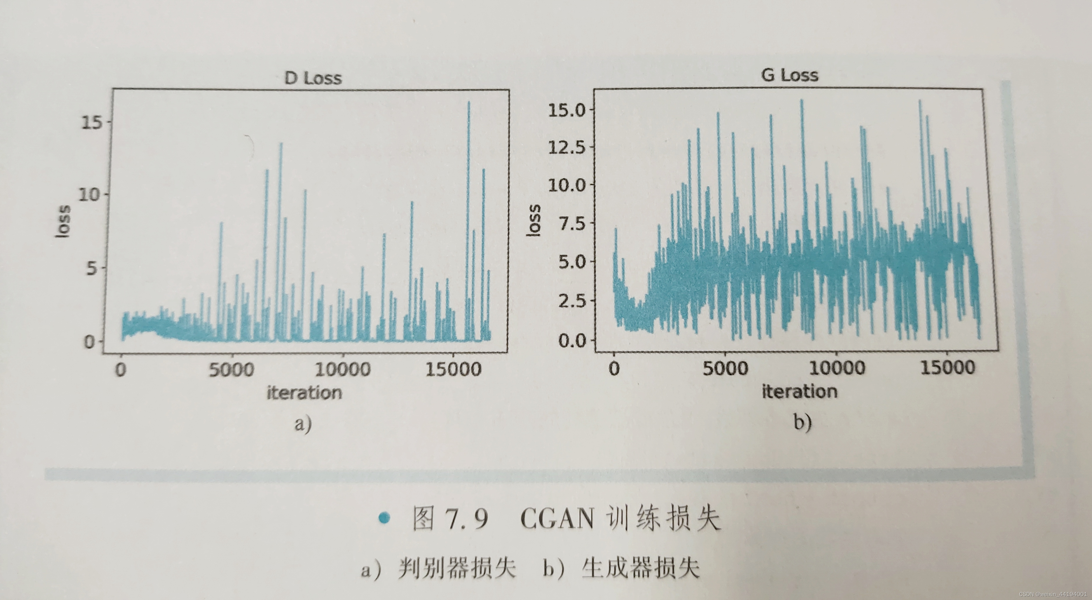
6.训练过程运行结果

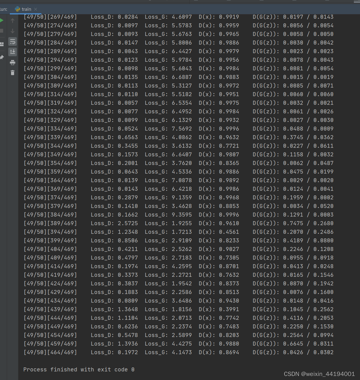
errD.item()和errG.item()分别是判别器和生成器的损失值。在这里，使用的是二元交叉熵损失函数（Binary Cross Entropy），因此这些损失值可以理解为交叉熵。

D_x表示判别器对于真实样本的输出均值，即真实样本被判别为真实样本的概率。

D_G_z1应该表示的是生成器生成的样本被判别成假样本的概率，因为label里面是fake_label,fake_label=0,即这一步应该是让判别器学会判别生成器生成的图片是虚假图片。

D_G_z2表示生成器生成的样本被判别为真实样本的概率。

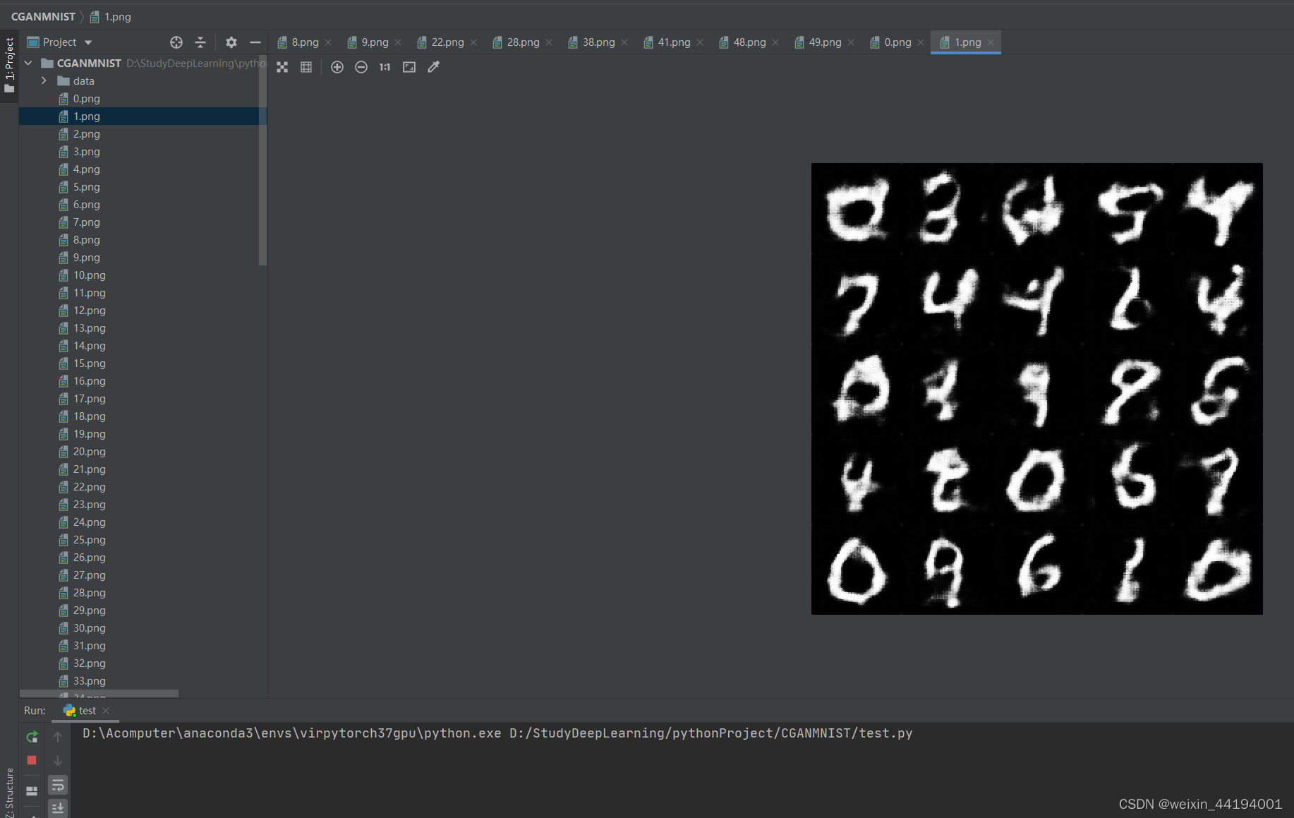
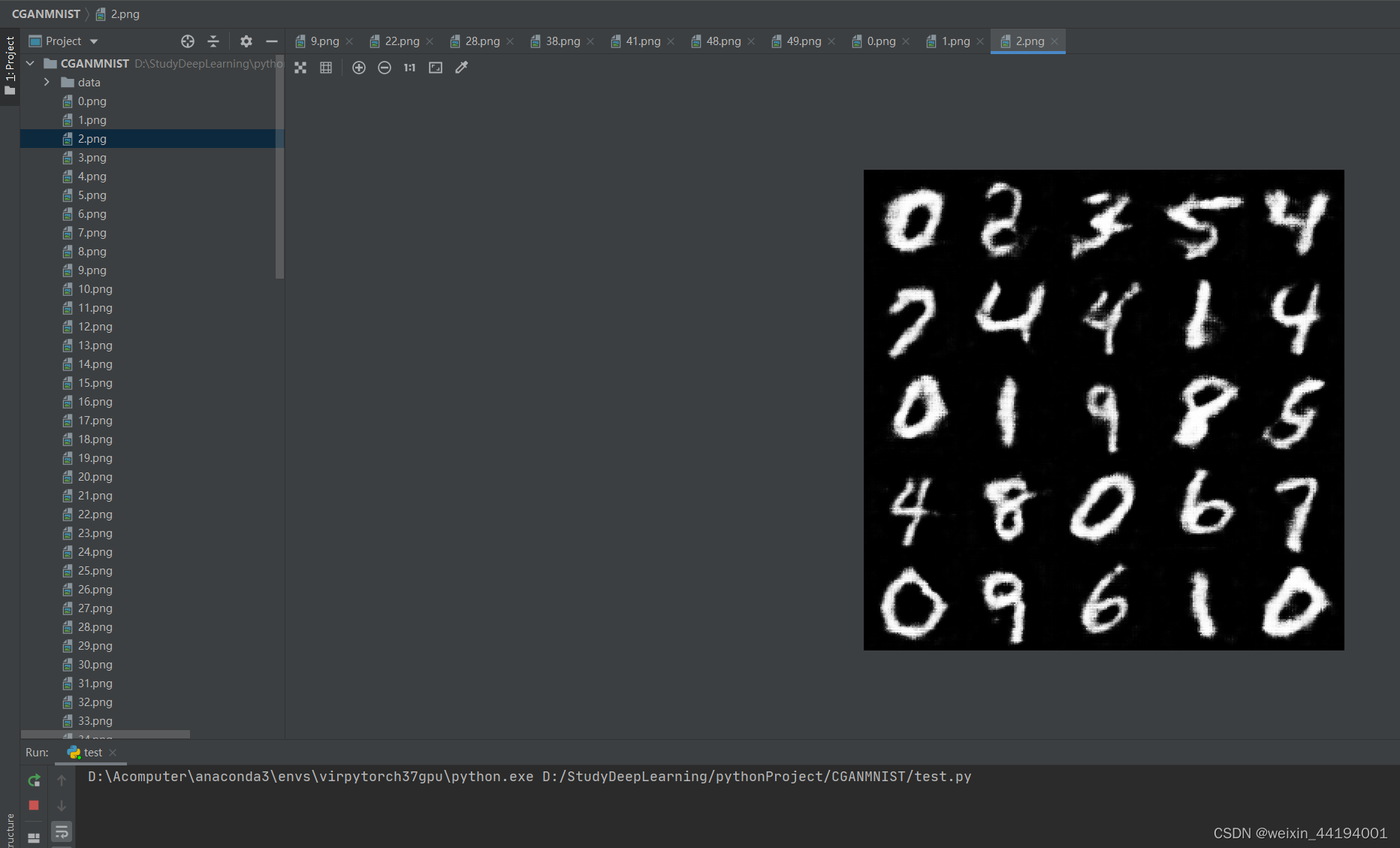
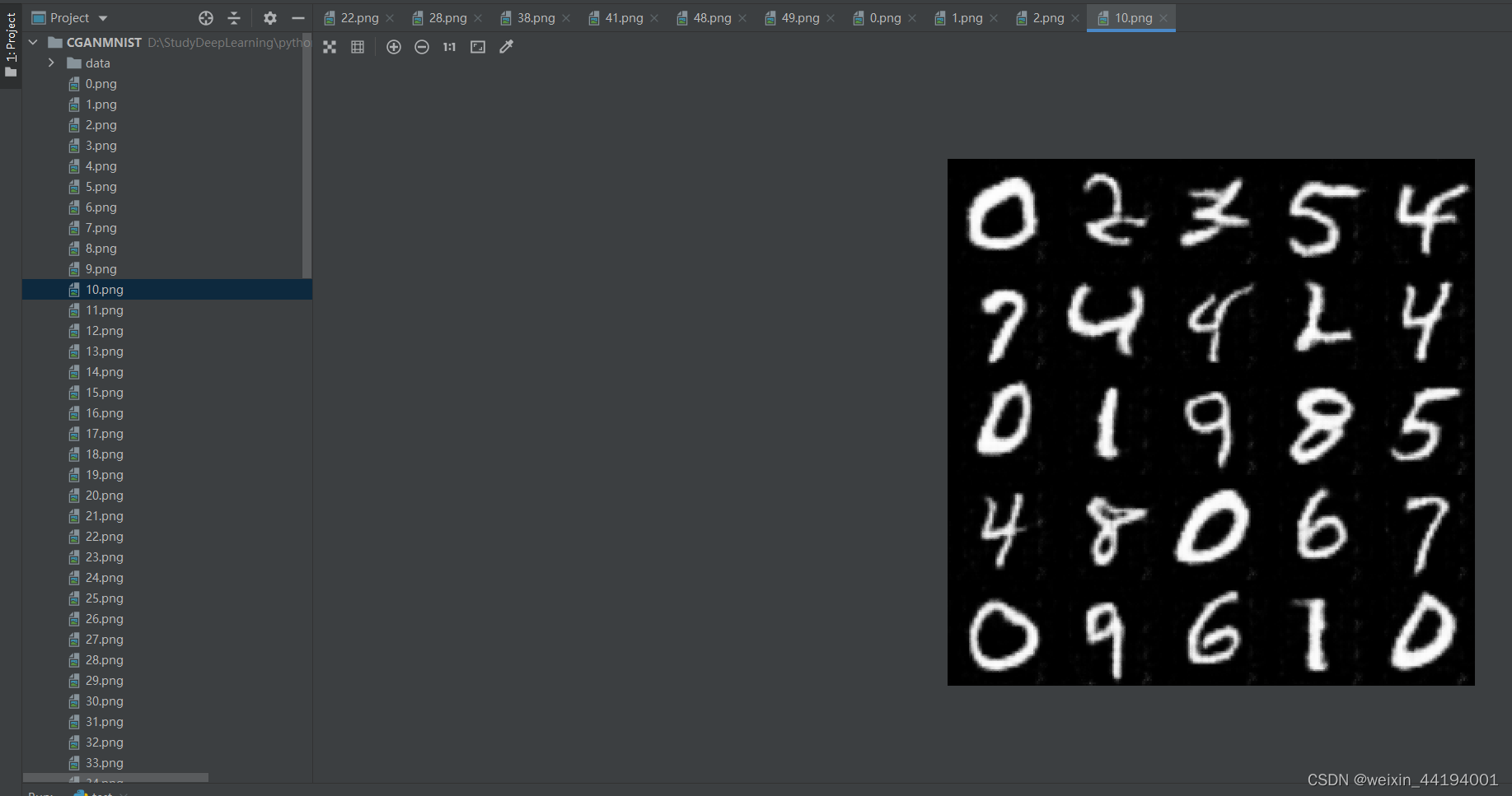
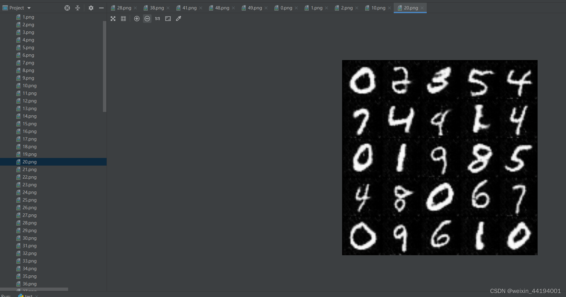
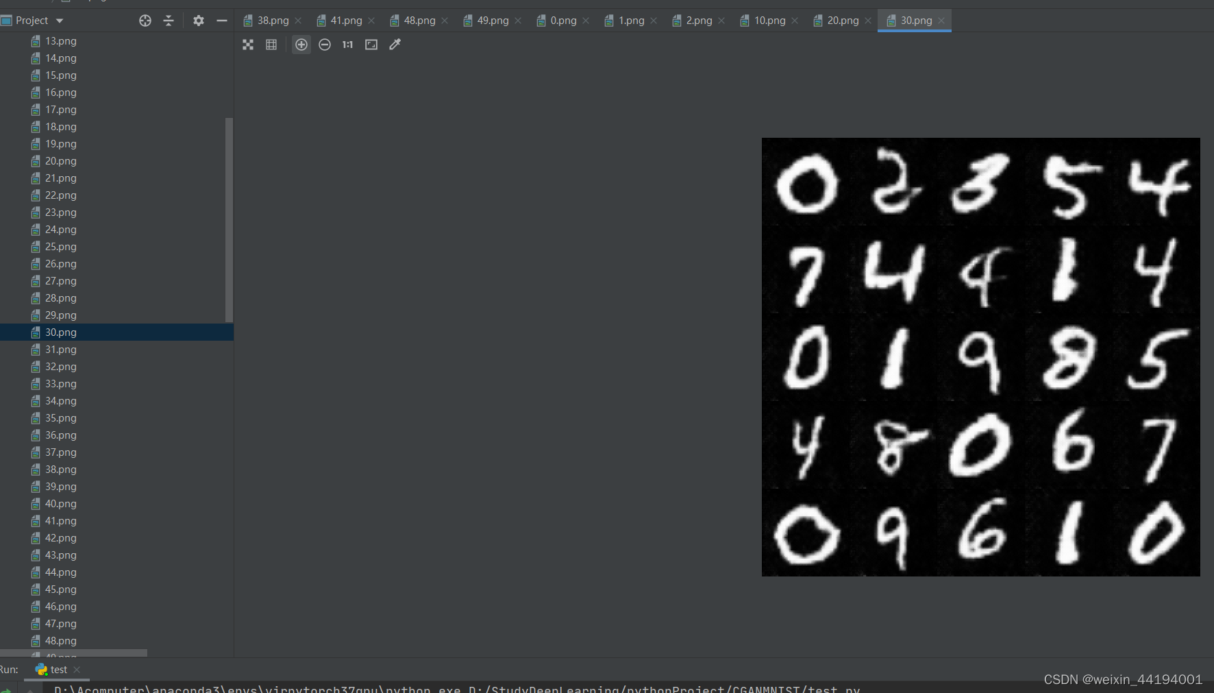
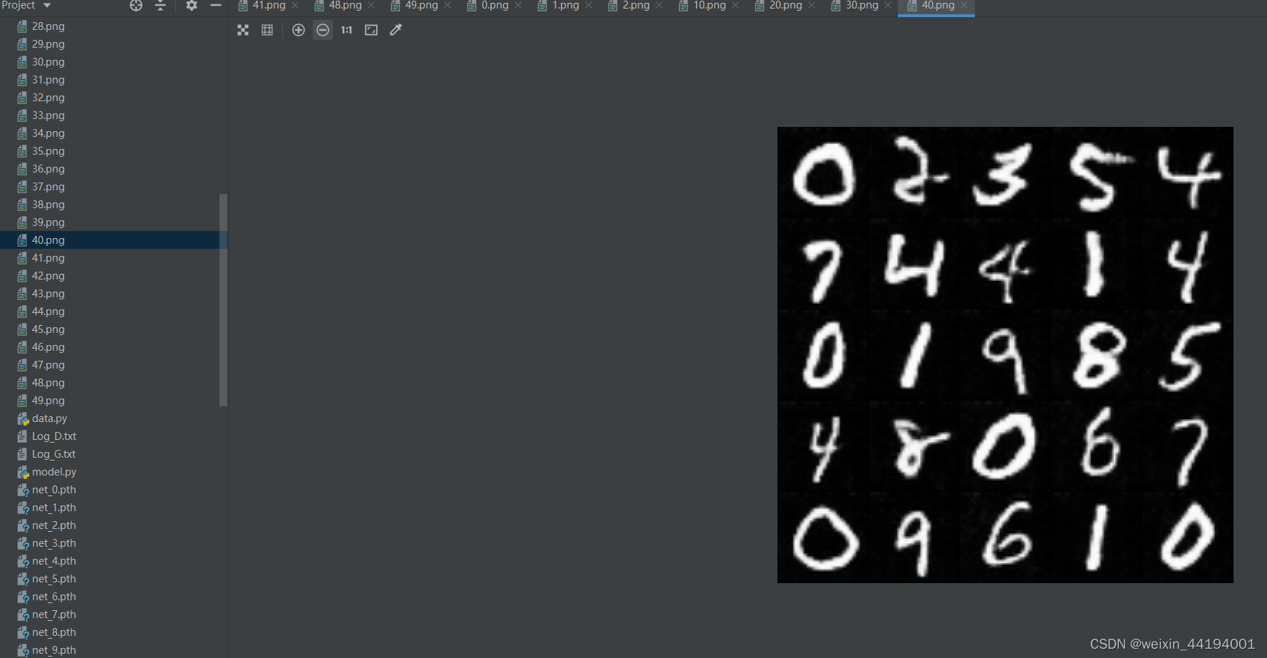
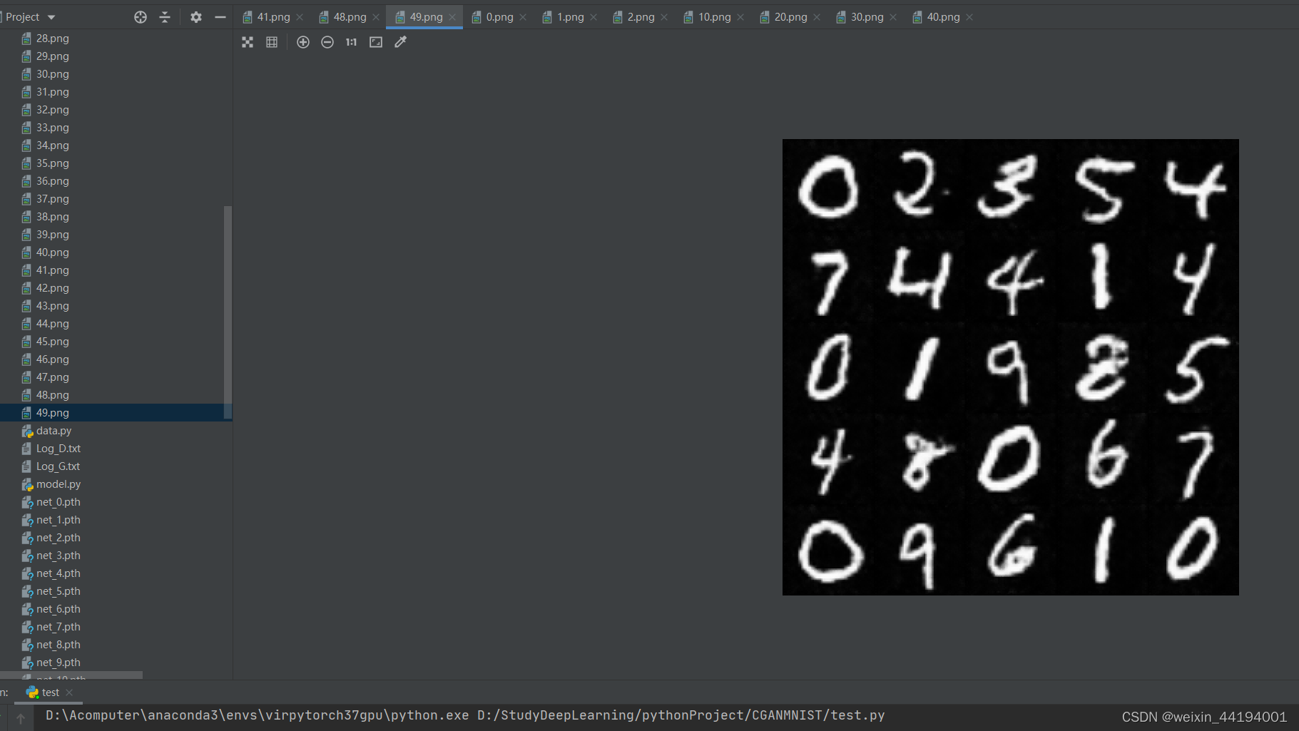
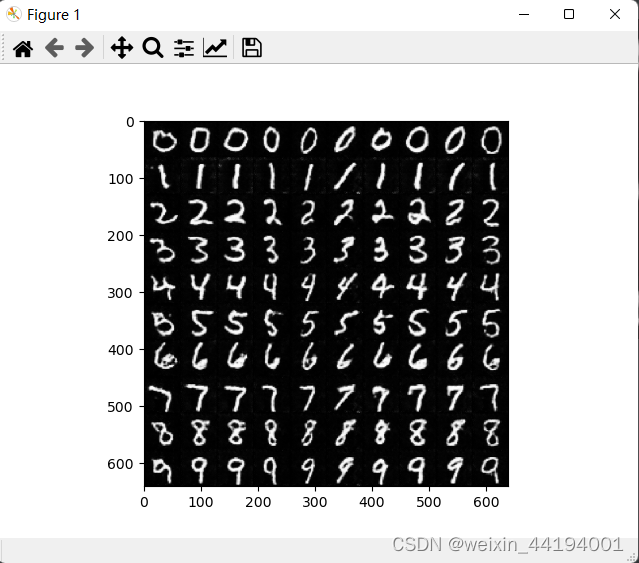
7.测试结果

测试代码

 NZ = 100 NUM_CLASS = 10 BATCH_SIZE = 10 DEVICE = "cpu" # fix_input_c = (torch.rand(BATCH_SIZE, 1) * NUM_CLASS).type(torch.LongTensor).squeeze().to(DEVICE) netG = Generator() netG = restore_network("./", "49", netG) fix_noise = torch.randn(BATCH_SIZE, NZ, device=DEVICE) fix_input_c = torch.tensor([0, 0, 0, 0, 0, 0, 0, 0, 0, 0]) device = "cuda" if torch.cuda.is_available() else "cpu" fix_input_c = onehot(fix_input_c, NUM_CLASS) fix_input_c = fix_input_c.to(device) fix_noise = fix_noise.to(device) netG = netG.to(device) #fake_imgs = netG(fix_noise, fix_input_c).detach().cpu() # images = recover_image(fake_imgs) # full_image = np.full((1 * 64, 10 * 64, 3), 0, dtype="uint8") # for i in range(10): # row = i // 10 # col = i % 10 # full_image[row * 64:(row + 1) * 64, col * 64:(col + 1) * 64, :] = images[i] #fix_noise = torch.randn(BATCH_SIZE, NZ, device=DEVICE) full_image = np.full((10 * 64, 10 * 64, 3), 0, dtype="uint8") for num in range(10): input_c = torch.tensor(np.ones(10, dtype="int64") * num) input_c = onehot(input_c, NUM_CLASS) fix_noise = fix_noise.to(device) input_c = input_c.to(device) fake_imgs = netG(fix_noise, input_c).detach().cpu() images = recover_image(fake_imgs) for i in range(10): row = num col = i % 10 full_image[row * 64:(row + 1) * 64, col * 64:(col + 1) * 64, :] = images[i] plt.imshow(full_image) plt.show() plt.imsave("hah.png", full_image)