讯享网

甲基化系列分析教程

桓峰基因公众号推出甲基化系列分析教程，整理如下：

甲基化系列 1. 甲基化之前世今生（Methylation）

甲基化系列 2. 甲基化芯片数据介绍与下载（GEO）

甲基化系列 3. 甲基化芯片数据分析完整版（ChAMP）

简介

DNA 甲基化特征通常是基于多元的方法，需要数以百计的预测网站。在这里，我们提出了一个计算框架 CimpleG 用于检测 CpG 甲基化特征，用于细胞类型分类功能和反卷积。CimpleG 既具有时间效率，又具有执行能力以及表现最好的血细胞和其他细胞类型分类方法而它的预测是基于每种细胞类型的单个 DNA 甲基化位点。总之，CimpleG 为描述提供了一个完整的计算框架 DNA 特征和细胞反褶积。

(A) 对用于特性选择和下游应用程序的 CimpleG 和统计的概述。体细胞(B)或白细胞(C)的DNAm数据集的主成分分析。训练样本(≥10个阳性样本)和测试数据的粗体突出显示的细胞类型被用作目标类。测试数据中不存在的细胞类型仅用作阴性示例(非靶细胞)。

软件包安装

# Install directly from github: devtools::install_github("costalab/CimpleG") # Alternatively, downloading from our release page and installing it from a local source: # - ie navigating through your system install.packages(file.choose(), repos = NULL, type = "source") # - ie given a path to a local source install.packages("~/Downloads/CimpleG_0.0.5.XXXX.tar.gz", repos = NULL, type = "source") # or devtools::install_local("~/Downloads/CimpleG_0.0.5.XXXX.tar.gz")

数据读取

讯享网library("CimpleG") data(train_data) train_data[1:5,1:5] cg cg0 cg0 cg cg0 GSM 0. 0. 0. 0. 0. GSM 0. 0. 0. 0. 0. GSM 0. 0. 0. 0. 0. GSM 0. 0. 0. 0. 0. GSM 0. 0. 0. 0. 0. data(train_targets) head(train_targets) gsm cell_type adipocytes astrocytes blood_cells 1 GSM endothelial_cells 0 0 0 2 GSM endothelial_cells 0 0 0 3 GSM endothelial_cells 0 0 0 4 GSM endothelial_cells 0 0 0 5 GSM endothelial_cells 0 0 0 6 GSM endothelial_cells 0 0 0 endothelial_cells epidermal_cells epithelial_cells fibroblasts glia 1 1 0 0 0 0 2 1 0 0 0 0 3 1 0 0 0 0 4 1 0 0 0 0 5 1 0 0 0 0 6 1 0 0 0 0 hepatocytes ips_cells msc muscle_cells neurons muscle_sc group_data 1 0 0 0 0 0 0 train 2 0 0 0 0 0 0 train 3 0 0 0 0 0 0 train 4 0 0 0 0 0 0 train 5 0 0 0 0 0 0 train 6 0 0 0 0 0 0 train description 1 ENDOTHELIAL.CELLS 2 ENDOTHELIAL.CELLS 3 ENDOTHELIAL.CELLS 4 ENDOTHELIAL.CELLS 5 ENDOTHELIAL.CELLS 6 ENDOTHELIAL.CELLS colnames(train_targets) [1] "gsm" "cell_type" "adipocytes" [4] "astrocytes" "blood_cells" "endothelial_cells" [7] "epidermal_cells" "epithelial_cells" "fibroblasts" [10] "glia" "hepatocytes" "ips_cells" [13] "msc" "muscle_cells" "neurons" [16] "muscle_sc" "group_data" "description" data(test_data) test_data[1:5,1:5] cg cg0 cg0 cg cg0 GSM 0.0 0. 0. 0. 0. GSM 0.0 0. 0. 0. 0. GSM 0. 0. 0. 0. 0. GSM 0. 0. 0. 0. 0. GSM 0. 0. 0. 0. 0. data(test_targets) # check the train_targets table to see # what other columns can be used as targets # colnames(train_targets)

实例操作

CimpleG试图找到对给定的训练数据集的细胞类型进行**分类的CpG, 还能够在几个简单的步骤中执行细胞型反褶积,可以使用beta值或M值。这里我们展示了生成signature就非常容易了。

运行 CimpleG

运行CimpleG非常简单。您只需要使用一些参数运行CimpleG函数。

# mini example with just 4 target signatures set.seed(42) cimpleg_result <- CimpleG( train_data = train_data, train_targets = train_targets, test_data = test_data, test_targets = test_targets, method = "CimpleG", target_columns = c( "neurons", "glia", "blood_cells", "fibroblasts" ) ) Training for target 'neurons' with 'CimpleG' has finished.: 1.63 sec elapsed Training for target 'glia' with 'CimpleG' has finished.: 0.5 sec elapsed Training for target 'blood_cells' with 'CimpleG' has finished.: 0.37 sec elapsed Training for target 'fibroblasts' with 'CimpleG' has finished.: 0.36 sec elapsed cimpleg_result$results $neurons $neurons$train_res $neurons$train_res$fold_id # A tibble: 4,090 × 3 Row Data Fold <int> <chr> <chr> 1 1 Analysis Fold02 2 1 Analysis Fold03 3 1 Analysis Fold04 4 1 Analysis Fold05 5 1 Analysis Fold06 6 1 Analysis Fold07 7 1 Analysis Fold08 8 1 Analysis Fold09 9 1 Analysis Fold10 10 2 Analysis Fold01 # ℹ 4,080 more rows $neurons$train_res$train_summary id stat_origin mean_aupr mean_var_a fold_presence 1: cg0 train_aupr 1.0000000 0.0 10 2: cg0 validation_aupr 1.0000000 0.0 10 3: cg train_aupr 1.0000000 0.0 10 4: cg validation_aupr 1.0000000 0.0 10 5: cg train_aupr 0. 0.0 10 6: cg validation_aupr 0. 0.0 10 7: cg train_aupr 0. 0.0 8 8: cg validation_aupr 1.0000000 0.0 8 9: cg train_aupr 1.0000000 0.0 10 10: cg validation_aupr 1.0000000 0.0 10 $neurons$train_res$dt_dmsv id diff_means sum_variance pred_type 1: cg0 -0. 0.00 FALSE 2: cg -0. 0.0 FALSE 3: cg -0. 0.0 FALSE 4: cg -0. 0.00 FALSE 5: cg 0. 0.00 TRUE $neurons$train_res$train_results id fold_presence diff_means sum_variance pred_type mean_var_a 1: cg 10 0. 0.00 TRUE 0.0 2: cg 10 -0. 0.0 FALSE 0.0 3: cg0 10 -0. 0.00 FALSE 0.0 4: cg 10 -0. 0.0 FALSE 0.0 5: cg 8 -0. 0.00 FALSE 0.0 train_aupr validation_aupr cpg_score train_rank 1: 1.0000000 1.0000000 0.00 1 2: 0. 0. 0.00 2 3: 1.0000000 1.0000000 0.00 3 4: 1.0000000 1.0000000 0.00 4 5: 0. 1.0000000 0.00 5 $neurons$test_perf id fold_presence diff_means sum_variance pred_type mean_var_a 1: cg 10 0. 0.00 TRUE 0.0 2: cg 10 -0. 0.0 FALSE 0.0 3: cg0 10 -0. 0.00 FALSE 0.0 4: cg 10 -0. 0.0 FALSE 0.0 5: cg 8 -0. 0.00 FALSE 0.0 train_mean_aupr validation_mean_aupr cpg_score train_rank test_aupr 1: 1.0000000 1.0000000 0.00 1 0. 2: 0. 0. 0.00 2 1.0000000 3: 1.0000000 1.0000000 0.00 3 0. 4: 1.0000000 1.0000000 0.00 4 0. 5: 0. 1.0000000 0.00 5 0. $neurons$elapsed_time Time difference of 1. secs $glia $glia$train_res $glia$train_res$fold_id # A tibble: 4,090 × 3 Row Data Fold <int> <chr> <chr> 1 1 Analysis Fold01 2 1 Analysis Fold02 3 1 Analysis Fold03 4 1 Analysis Fold05 5 1 Analysis Fold06 6 1 Analysis Fold07 7 1 Analysis Fold08 8 1 Analysis Fold09 9 1 Analysis Fold10 10 2 Analysis Fold01 # ℹ 4,080 more rows $glia$train_res$train_summary id stat_origin mean_aupr mean_var_a fold_presence 1: cg0 train_aupr 1.0000000 0.0 10 2: cg0 validation_aupr 1.0000000 0.0 10 3: cg0 train_aupr 0. 0.0 10 4: cg0 validation_aupr 0. 0.0 10 5: cg train_aupr 0. 0.0 10 6: cg validation_aupr 0. 0.0 10 7: cg train_aupr 1.0000000 0.0 10 8: cg validation_aupr 1.0000000 0.0 10 9: cg train_aupr 0. 0.0 10 10: cg validation_aupr 1.0000000 0.0 10 $glia$train_res$dt_dmsv id diff_means sum_variance pred_type 1: cg0 -0. 0.0 FALSE 2: cg0 -0. 0.00 FALSE 3: cg -0. 0.00 FALSE 4: cg -0. 0.00 FALSE 5: cg -0. 0.00 FALSE $glia$train_res$train_results id fold_presence diff_means sum_variance pred_type mean_var_a 1: cg 10 -0. 0.00 FALSE 0.0 2: cg0 10 -0. 0.0 FALSE 0.0 3: cg 10 -0. 0.00 FALSE 0.0 4: cg 10 -0. 0.00 FALSE 0.0 5: cg0 10 -0. 0.00 FALSE 0.0 train_aupr validation_aupr cpg_score train_rank 1: 1.0000000 1.000 0.00 1 2: 1.0000000 1.000 0.00 2 3: 0. 1.000 0.00 3 4: 0. 0.925 0.00 4 5: 0. 0.775 0.00 5 $glia$test_perf id fold_presence diff_means sum_variance pred_type mean_var_a 1: cg 10 -0. 0.00 FALSE 0.0 2: cg0 10 -0. 0.0 FALSE 0.0 3: cg 10 -0. 0.00 FALSE 0.0 4: cg 10 -0. 0.00 FALSE 0.0 5: cg0 10 -0. 0.00 FALSE 0.0 train_mean_aupr validation_mean_aupr cpg_score train_rank test_aupr 1: 1.0000000 1.000 0.00 1 0. 2: 1.0000000 1.000 0.00 2 0. 3: 0. 1.000 0.00 3 1.0000000 4: 0. 0.925 0.00 4 1.0000000 5: 0. 0.775 0.00 5 0. $glia$elapsed_time Time difference of 0. secs $blood_cells $blood_cells$train_res $blood_cells$train_res$fold_id # A tibble: 4,090 × 3 Row Data Fold <int> <chr> <chr> 1 1 Analysis Fold01 2 1 Analysis Fold02 3 1 Analysis Fold03 4 1 Analysis Fold04 5 1 Analysis Fold05 6 1 Analysis Fold06 7 1 Analysis Fold08 8 1 Analysis Fold09 9 1 Analysis Fold10 10 2 Analysis Fold01 # ℹ 4,080 more rows $blood_cells$train_res$train_summary id stat_origin mean_aupr mean_var_a fold_presence 1: cg0 train_aupr 0. 0.0 10 2: cg0 validation_aupr 0. 0.0 10 3: cg0 train_aupr 0. 0.0 10 4: cg0 validation_aupr 0. 0.0 10 5: cg0 train_aupr 0. 0.0 10 6: cg0 validation_aupr 0. 0.0 10 7: cg train_aupr 0. 0.0 10 8: cg validation_aupr 0. 0.0 10 9: cg train_aupr 0. 0.0 10 10: cg validation_aupr 0. 0.0 10 $blood_cells$train_res$dt_dmsv id diff_means sum_variance pred_type 1: cg0 -0. 0.0 FALSE 2: cg0 -0. 0.0 FALSE 3: cg0 0. 0.0 TRUE 4: cg 0. 0.0 TRUE 5: cg 0. 0.0 TRUE $blood_cells$train_res$train_results id fold_presence diff_means sum_variance pred_type mean_var_a 1: cg0 10 -0. 0.0 FALSE 0.0 2: cg0 10 -0. 0.0 FALSE 0.0 3: cg 10 0. 0.0 TRUE 0.0 4: cg 10 0. 0.0 TRUE 0.0 5: cg0 10 0. 0.0 TRUE 0.0 train_aupr validation_aupr cpg_score train_rank 1: 0. 0. 0.00 1 2: 0. 0. 0.00 2 3: 0. 0. 0.00 3 4: 0. 0. 0.00 4 5: 0. 0. 0.00 5 $blood_cells$test_perf id fold_presence diff_means sum_variance pred_type mean_var_a 1: cg0 10 -0. 0.0 FALSE 0.0 2: cg0 10 -0. 0.0 FALSE 0.0 3: cg 10 0. 0.0 TRUE 0.0 4: cg 10 0. 0.0 TRUE 0.0 5: cg0 10 0. 0.0 TRUE 0.0 train_mean_aupr validation_mean_aupr cpg_score train_rank test_aupr 1: 0. 0. 0.00 1 0. 2: 0. 0. 0.00 2 0. 3: 0. 0. 0.00 3 0. 4: 0. 0. 0.00 4 0. 5: 0. 0. 0.00 5 0. $blood_cells$elapsed_time Time difference of 0. secs $fibroblasts $fibroblasts$train_res $fibroblasts$train_res$fold_id # A tibble: 4,090 × 3 Row Data Fold <int> <chr> <chr> 1 1 Analysis Fold01 2 1 Analysis Fold02 3 1 Analysis Fold04 4 1 Analysis Fold05 5 1 Analysis Fold06 6 1 Analysis Fold07 7 1 Analysis Fold08 8 1 Analysis Fold09 9 1 Analysis Fold10 10 2 Analysis Fold01 # ℹ 4,080 more rows $fibroblasts$train_res$train_summary id stat_origin mean_aupr mean_var_a fold_presence 1: cg0 train_aupr 0. 0. 5 2: cg0 validation_aupr 0. 0. 5 3: cg0 train_aupr 0. 0. 10 4: cg0 validation_aupr 0. 0. 10 5: cg0 train_aupr 0. 0. 10 6: cg0 validation_aupr 0. 0. 10 7: cg0 train_aupr 0. 0. 9 8: cg0 validation_aupr 0. 0. 9 9: cg train_aupr 0. 0. 6 10: cg validation_aupr 0. 0. 6 $fibroblasts$train_res$dt_dmsv id diff_means sum_variance pred_type 1: cg0 -0. 0.0 FALSE 2: cg0 -0. 0.0 FALSE 3: cg0 -0. 0. FALSE 4: cg0 -0. 0.0 FALSE 5: cg -0. 0. FALSE $fibroblasts$train_res$train_results id fold_presence diff_means sum_variance pred_type mean_var_a 1: cg0 10 -0. 0. FALSE 0. 2: cg0 10 -0. 0.0 FALSE 0. 3: cg0 9 -0. 0.0 FALSE 0. 4: cg 6 -0. 0. FALSE 0. 5: cg0 5 -0. 0.0 FALSE 0. train_aupr validation_aupr cpg_score train_rank 1: 0. 0. 0.0 1 2: 0. 0. 0.0 2 3: 0. 0. 0.0 3 4: 0. 0. 0.0 4 5: 0. 0. 0.0 5 $fibroblasts$test_perf id fold_presence diff_means sum_variance pred_type mean_var_a 1: cg0 10 -0. 0. FALSE 0. 2: cg0 10 -0. 0.0 FALSE 0. 3: cg0 9 -0. 0.0 FALSE 0. 4: cg 6 -0. 0. FALSE 0. 5: cg0 5 -0. 0.0 FALSE 0. train_mean_aupr validation_mean_aupr cpg_score train_rank test_aupr 1: 0. 0. 0.0 1 0. 2: 0. 0. 0.0 2 0. 3: 0. 0. 0.0 3 0. 4: 0. 0. 0.0 4 0. 5: 0. 0. 0.0 5 0. $fibroblasts$elapsed_time Time difference of 0. secs # adjust target names to match signature names

绘制 CimpleG CpG signature

讯享网# check generated signatures plt <- signature_plot( cimpleg_result, train_data, train_targets, sample_id_column = "gsm", true_label_column = "cell_type" ) print(plt$plot)

均值之差与方差和(dmsv)图

基本的绘图

plt <- diffmeans_sumvariance_plot( data = train_data, target_vector = train_targets$neurons == 1 ) print(plt)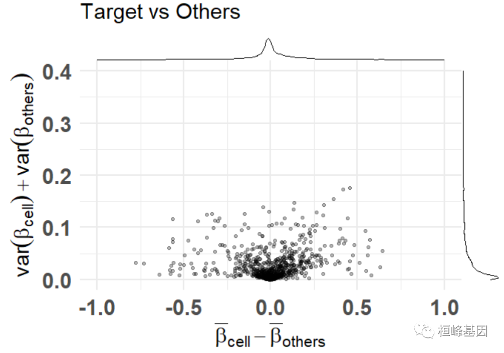

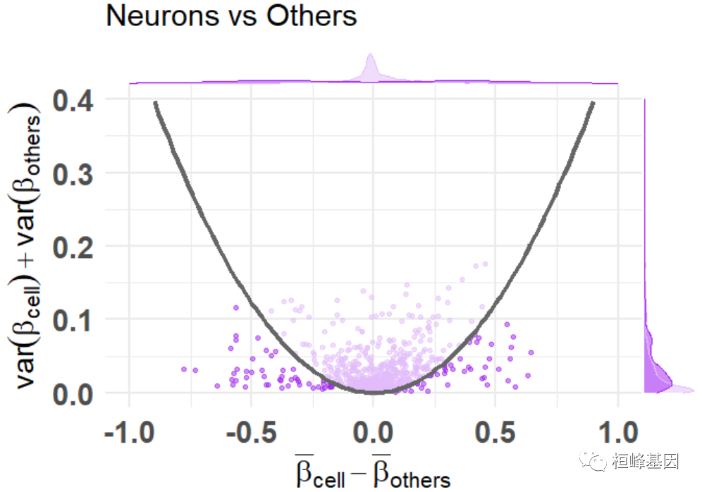
添加颜色，突出显示选定的功能

讯享网df_dmeansvar <- compute_diffmeans_sumvar( data = train_data, target_vector = train_targets$neurons == 1 ) parab_param <- .7 df_dmeansvar$is_selected <- select_features( x = df_dmeansvar$diff_means, y = df_dmeansvar$sum_variance, a = parab_param ) plt <- diffmeans_sumvariance_plot( data = df_dmeansvar, label_var1 = "Neurons", color_all_points = "purple", threshold_func = function(x, a) (a * x) ^ 2, is_feature_selected_col = "is_selected", func_factor = parab_param ) print(plt)

标记特征基因

plt <- diffmeans_sumvariance_plot( data = df_dmeansvar, feats_to_highlight = cimpleg_result$signatures ) print(plt)

绘制反卷积图

最小的例子只有4个signature

讯享网deconv_result <- run_deconvolution( cpg_obj = cimpleg_result, new_data = test_data ) plt <- deconvolution_barplot( deconvoluted_data = deconv_result, meta_data = test_targets, sample_id = "gsm", true_label = "cell_type" ) print(plt$plot)

更高级的例子

这个例子更高级一些。首先，创建额外的反卷积结果，以便我们可以比较，使用CimpleG创建另外两个模型。一种只使用高甲基化的特征，另一种每个特征使用3个CpGs，而不是一个。

set.seed(42) cimpleg_hyper <- CimpleG( train_data = train_data, train_targets = train_targets, test_data = test_data, test_targets = test_targets, method = "CimpleG", pred_type = "hyper", target_columns = c( "neurons", "glia", "blood_cells", "fibroblasts" ) ) Training for target 'neurons' with 'CimpleG' has finished.: 0.48 sec elapsed Training for target 'glia' with 'CimpleG' has finished.: 0.28 sec elapsed Training for target 'blood_cells' with 'CimpleG' has finished.: 0.33 sec elapsed Training for target 'fibroblasts' with 'CimpleG' has finished.: 0.28 sec elapsed deconv_hyper <- run_deconvolution( cpg_obj = cimpleg_hyper, new_data = test_data ) set.seed(42) cimpleg_3sigs <- CimpleG( train_data = train_data, train_targets = train_targets, test_data = test_data, test_targets = test_targets, method = "CimpleG", n_sigs = 3, target_columns = c( "neurons", "glia", "blood_cells", "fibroblasts" ) ) Training for target 'neurons' with 'CimpleG' has finished.: 0.38 sec elapsed Training for target 'glia' with 'CimpleG' has finished.: 0.36 sec elapsed Training for target 'blood_cells' with 'CimpleG' has finished.: 0.37 sec elapsed Training for target 'fibroblasts' with 'CimpleG' has finished.: 0.5 sec elapsed deconv_3sigs <- run_deconvolution( cpg_obj = cimpleg_3sigs, new_data = test_data )

让我们也创建一些假的真值，以便我们可以比较所有的结果。记住这只是一个例子，结果本身是没有意义的!

讯享网deconv_3sigs$prop_3sigs <- deconv_3sigs$proportion deconv_hyper$prop_hyper <- deconv_hyper$proportion deconv_result$prop_cimpleg <- deconv_result$proportion dummy_deconvolution_data <- deconv_result |> dplyr::mutate(true_vals = proportion + runif(nrow(deconv_result), min=-0.1,max=0.1)) |> dplyr::select(cell_type,sample_id,prop_cimpleg,true_vals) |> dplyr::left_join(deconv_hyper |> dplyr::select(-proportion), by=c("sample_id","cell_type")) |> dplyr::left_join(deconv_3sigs |> dplyr::select(-proportion), by=c("sample_id","cell_type")) |> dplyr::mutate_if(is.numeric, function(x){ifelse(x<0,0,x)}) |> dplyr::mutate_if(is.numeric, function(x){ifelse(x>1,1,x)}) |> tibble::as_tibble()

现在让我们利用一些用来比较反卷积结果的绘图函数，我们可以检查真实值与预测值的比较。

install.packages("broom") 程序包'broom'打开成功，MD5和检查也通过 下载的二进制程序包在 C:\Users\Lenovo\AppData\Local\Temp\RtmpOonYSV\downloaded_packages里 scatter_plts <- CimpleG:::deconv_pred_obs_plot( deconv_df = dummy_deconvolution_data, true_values_col = "true_vals", predicted_cols = c("prop_cimpleg","prop_hyper","prop_3sigs"), sample_id_col = "sample_id", group_col= "cell_type" ) scatter_panel <- scatter_plts |> patchwork::wrap_plots(ncol=1) print(scatter_panel)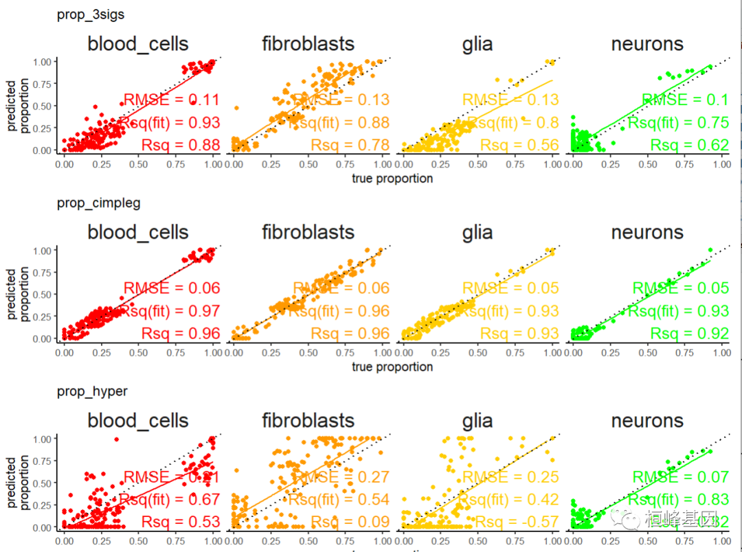

现在，更有趣的是，我们可以详细地看到并对用于评估反卷积结果的一个措施进行排序。

讯享网rank_plts <- CimpleG:::deconv_ranking_plot( deconv_df = dummy_deconvolution_data, true_values_col = "true_vals", predicted_cols = c("prop_cimpleg","prop_hyper","prop_3sigs"), sample_id_col = "sample_id", group_col= "cell_type", metrics = "rmse" ) rank_panel <- list(rank_plts$perf_boxplt[[1]],rank_plts$nemenyi_plt[[1]]) |> patchwork::wrap_plots() print(rank_panel)

Reference

1. Maié T, Schmidt M, Erz M, Wagner W, G Costa I. CimpleG: finding simple CpG methylation signatures. Genome Biol. 2023 Jul 10;24(1):161. doi: 10.1186/s13059-023-03000-0. PMID: ; PMCID: PMC.

桓峰基因，铸造成功的您！

未来桓峰基因公众号将不间断的推出单细胞系列生信分析教程，

敬请期待！！

桓峰基因官网正式上线，请大家多多关注，还有很多不足之处，大家多多指正！

http://www.kyohogene.com/

桓峰基因和投必得合作，文章润色优惠85折，需要文章润色的老师可以直接到网站输入领取桓峰基因专属优惠券码：KYOHOGENE，然后上传，付款时选择桓峰基因优惠券即可享受85折优惠哦！https://www.topeditsci.com/