Load package and time series

In this demonstration, we use the same time series generated from the 5-species model (Resource, Consumer1, Consumer2, Predator1, Predator2) following Deyle et al. (2016).

 Load package and data library(rEDM) d <- read.csv("ESM5_Data_5spModel.csv") 

Set parameters and do S-map

In this demonstration, we focus on the effects on Consumer1 (C1). As shown in Deyle et al. (2016), the effects of Predator2 (P2) on C1 are negligible, and thus we ignore P2 in the embedding. We use fully multivariate embedding (Deyle et al. 2016, Deyle et al. 2011) in order to investigate effects of R, C2, and P1 on C1.

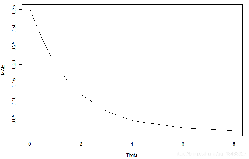
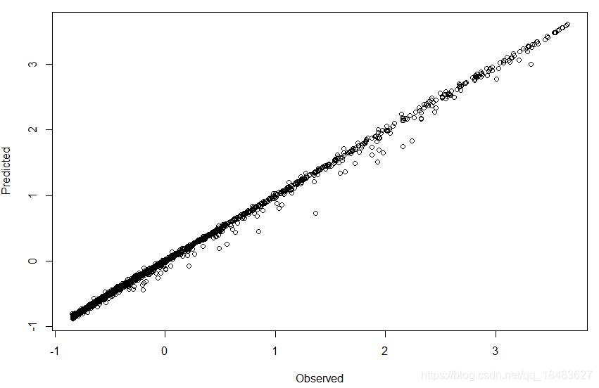
讯享网# Make multivariate embedding Embedding <- c("R","C1","C2","P1") block <- d[,Embedding] # Normalize data block <- as.data.frame(apply(block, 2, function(x) (x-mean(x))/sd(x))) # Define the target column (C1 = column 2) targ_col <- 2 # Please reduce the number of data points if the calculation takes long data_used <- 1:2000 # Explore the best weighting parameter (nonlinear parameter = theta) # Best theta is selected based on mean absolute error (MAE) test_theta <- block_lnlp(block[data_used,], method = "s-map", num_neighbors = 0, # We have to use any value < 1 for s-map theta = c(0, 1e-04, 3e-04, 0.001, 0.003, 0.01, 0.03, 0.1, 0.3, 0.5, 0.75, 1, 1.5, 2, 3, 4, 6, 8), # We try many thetas to find the best parameter target_column = targ_col, # Specify the target column silent = T) # Check MAE and theta plot(test_theta$mae~test_theta$theta, type="l", xlab="Theta", ylab="MAE") # Best theta = 8 in this case best_theta <- test_theta[which.min(test_theta$mae),"theta"] # Do S-map analysis with the best theta smap_res <- block_lnlp(block[data_used,], method = "s-map", num_neighbors = 0, # we have to use any value < 1 for s-map theta = best_theta, target_column = targ_col, silent = T, save_smap_coefficients = T) # save S-map coefficients Visualize results Observed v.s. Predicted smap_out <- as.data.frame(smap_res$model_output[[1]]) plot(smap_out$obs, smap_out$pred, xlab="Observed", ylab="Predicted") Time series of fluctuating interaction strength smap_coef <- as.data.frame(smap_res$smap_coefficients[[1]]) colnames(smap_coef) <- c("dC1dR","dC1dC1","dC1dC2","dC1dP1","Intercept") # Plot all partial derivatives trange <- 1:200 windows(width=6, height=4) plot(smap_coef[trange,"dC1dR"], type="l", col="royalblue", lwd=2, xlab="time", ylab="Interction strength", ylim = c(-1.0, 2.5), main = "Fluctuating interaction strength") lines(smap_coef[trange,"dC1dC2"], lwd=2, col="red3") lines(smap_coef[trange,"dC1dP1"], lwd=2, col="springgreen3") abline(a=0 ,b=0 , lty="dashed", col="black", lwd=.5)

修改了原代码中的一些小错误。

讯享网

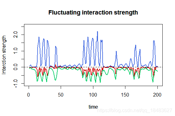
As can be seen in Figure 7 in the main text, interaction strengths fluctuate with time.

References

Deyle E, Sugihara G (2011) Generalized theorems for nonlinear state space reconstruction. PLoS ONE 6: e18295.(PDF)

Deyle ER, May RM, Munch SB, Sugihara G (2016) Tracking and forecasting ecosystem interactions in real time. Proc R Soc Lond B Biol Sci 283: .(PDF)