大家好，我是讯享网，很高兴认识大家。

本例程配套完整源码和数据集下载

目录：

一、下载训练、验证和测试数据

二、下载预训练网络和样本测试集

三、3-D U-Net 网络训练

四、执行测试数据的分割

五、dice量化分割精度

此示例展示了如何训练一个3-D U-Net 神经网络，并对三维磁共振成像(MRI)图像数据进行脑肿瘤的分割。

                                  
讯享网

一、下载训练、验证和测试数据

此示例使用 BraTS 数据集 ，包含脑部MRI 扫描的神经胶质瘤，这是最常见的原发性脑恶性肿瘤。数据文件的大小约为 7 GB。如果您不想下载 BraTS 数据集，则直接进入本示例中的下载预训练网络和样本测试集部分。

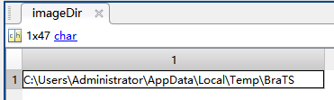
1.1 创建一个目录来存储 BraTS 数据集

%查找Windows系统上临时文件夹下是否有BraTS文件夹 imageDir = fullfile(tempdir,'BraTS');%BraTS文件夹的完整目录赋值给imageDir if ~exist(imageDir,'dir') mkdir(imageDir); %如果BraTS文件夹不存在则建立一个 end

讯享网

二、下载预训练网络和样本测试集

2.1 从 BraTS 数据集下载 3-D U-Net 的预训练版本和五个样本测试卷及其相应的标签。预训练模型和样本数据使您无需下载完整数据集或等待网络训练即可对测试数据执行分割

讯享网%3-D U-Net预训练模型下载地址 trained3DUnet_url = 'https://www.mathworks.com/supportfiles/vision/data/brainTumor3DUNetValid.mat'; %样本数据下载地址 sampleData_url = 'https://www.mathworks.com/supportfiles/vision/data/sampleBraTSTestSetValid.tar.gz'; %查找Windows系统是否有BraTS文件夹 imageDir = fullfile(tempdir,'BraTS');%BraTS文件夹的完整目录赋值给imageDir if ~exist(imageDir,'dir') mkdir(imageDir); %如果BraTS文件夹不存在则建立一个 end %加载3-D U-Net网络模型和五份mat测试样本数据(包含原图像测试数据和对应的标签测试数据) downloadTrained3DUnetSampleData(trained3DUnet_url,sampleData_url,imageDir);

2.2 建立的空文件夹BraTS目录

2.3 下载过程需要等待几分钟：

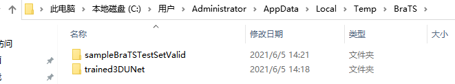
2.4 下载完成后预训练模型和样本数据便可以在BraTS文件夹中看到：

2.5 mat格式的预训练模型：

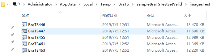
2.6 五份mat格式的测试样本的原图像数据：

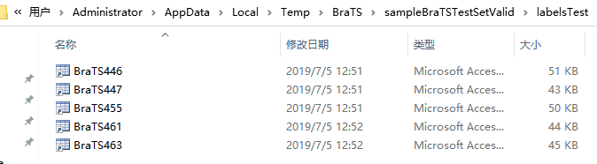
2.7 五份mat格式的测试样本的标签(Labels)数据：

三、3-D U-Net 网络训练

3.1 默认情况下，该示例加载一个预处理的3-D U-Net 网络。预训练网络使您能够运行整个示例，而无需等待训练完成。如果要训练网络，请将下面代码中的doTraining变量设置为true。使用训练网络(深度学习工具箱)功能训练模型。如果有图形处理器，就在上面训练。使用图形处理器需要并行计算工具箱和支持CUDA的NVIDIA图形处理器。

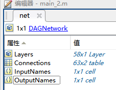
%%3-D U-Net网络训练 doTraining = false;%是否要训练网络(false or true) if doTraining modelDateTime = string(datetime('now','Format',"yyyy-MM-dd-HH-mm-ss")); [net,info] = trainNetwork(dsTrain,lgraph,options); save(strcat("trained3DUNet-",modelDateTime,"-Epoch-",num2str(options.MaxEpochs),".mat"),'net'); else inputPatchSize = [132 132 132 4]; outPatchSize = [44 44 44 2]; %加载3-D U-Net网络模型和五份mat测试样本数据(包含原图像测试数据和对应的标签测试数据) load(fullfile(imageDir,'trained3DUNet','brainTumor3DUNetValid.mat')); end

3.2 加载后的3-D U-Net网络预训练模型：

四、执行测试数据的分割

强烈建议使用 GPU 来执行图像体的语义分割（需要 Parallel Computing Toolbox™）。

4.1 选择包含真实图像体和包含测试标签的测试数据源进行测试。如果您将以下代码中的useFullTestSet变量修改为false，则该示例将使用5个图像体进行测试。如果您将useFullTestSet变量设置为true，则该示例使用从完整数据集中选择 55 个测试图像进行测试。

讯享网%执行测试数据的分割 %false：只使用BraTS文件夹下的5个测试数据进行测试 %true：使用preprocessDataLoc文件夹下的所有55个测试数据进行测试 useFullTestSet = false; if useFullTestSet volLocTest = fullfile(preprocessDataLoc,'imagesTest'); lblLocTest = fullfile(preprocessDataLoc,'labelsTest'); else %加载原图像测试数据路径 volLocTest = fullfile(imageDir,'sampleBraTSTestSetValid','imagesTest'); %加载标签测试数据路径 lblLocTest = fullfile(imageDir,'sampleBraTSTestSetValid','labelsTest'); %背景 肿瘤 classNames = ["background","tumor"]; pixelLabelID = [0 1]; end

4.2 voldsTest 变量存储真实值测试图像。pxdsTest 变量存储真实值标签

volReader = @(x) matRead(x); %使用 imageDatastore 函数为原图像创建图像文件集voldsTest对象 voldsTest = imageDatastore(volLocTest, ... 'FileExtensions','.mat','ReadFcn',volReader); %使用 imageDatastore 函数为标签图像创建pxdsTest对象 pxdsTest = pixelLabelDatastore(lblLocTest,classNames,pixelLabelID, ... 'FileExtensions','.mat','ReadFcn',volReader);

4.3 使用重叠分块策略来预测每个测试图像体的标签。对每个测试图像体都进行填充，以使输入大小是网络输出大小的倍数，并补偿有效卷积的效应。重叠分块算法选择重叠补片，使用 semanticseg (Computer Vision Toolbox) 函数预测每个补片的标签，然后重新组合补片。

讯享网%id=1表示第一份脑部数据（一份表示一个病人的整个系列切片数据） id = 1; while hasdata(voldsTest) %显示正在处理的数据号 disp(['Processing test volume ' num2str(id)]); %240*240*152的数据 加载标签图像数据大小 tempGroundTruth = read(pxdsTest); %240*240*152的数据 标签图像 groundTruthLabels{id} = tempGroundTruth{1}; %加载原图像数据，id表示对应第几份数据 vol{id} = read(voldsTest); %对测试图像使用反射填充 %避免填充不同的模态 volSize = size(vol{id},(1:3));%数据尺寸为240*240*152 %（132-44）/2 padSizePre = (inputPatchSize(1:3)-outPatchSize(1:3))/2; padSizePost = (inputPatchSize(1:3)-outPatchSize(1:3))/2 + (outPatchSize(1:3)-mod(volSize,outPatchSize(1:3))); volPaddedPre = padarray(vol{id},padSizePre,'symmetric','pre'); volPadded = padarray(volPaddedPre,padSizePost,'symmetric','post'); [heightPad,widthPad,depthPad,~] = size(volPadded); [height,width,depth,~] = size(vol{id}); %分割结果变量tempSeg tempSeg = categorical(zeros([height,width,depth],'uint8'),[0;1],classNames); % 用于体素分割的重叠平铺策略. for k = 1:outPatchSize(3):depthPad-inputPatchSize(3)+1 for j = 1:outPatchSize(2):widthPad-inputPatchSize(2)+1 for i = 1:outPatchSize(1):heightPad-inputPatchSize(1)+1 patch = volPadded( i:i+inputPatchSize(1)-1,... j:j+inputPatchSize(2)-1,... k:k+inputPatchSize(3)-1,:); patchSeg = semanticseg(patch,net); tempSeg(i:i+outPatchSize(1)-1, ... j:j+outPatchSize(2)-1, ... k:k+outPatchSize(3)-1) = patchSeg; end end end %裁剪掉多余的填充区域. tempSeg = tempSeg(1:height,1:width,1:depth); %保存预测的体积结果. predictedLabels{id} = tempSeg; %id进行累加表示处理更多份脑部数据 id=id+1; end

4.4 将真实值与网络预测进行比较。选择测试图像之一来评估语义分割的准确度。从四维体数据中提取第一个形态，并将此三维体存储在变量 vol3d 中

%表示第一份脑部数据 volId = 1; %获取原图像数据 大小为240*240*152 vol3d = vol{volId}(:,:,:,1);

4.5 使用蒙太奇显示该份数据中心切片的金标准图像和神经网络预测分割的图像

讯享网%vol3d的第三维维度/2 即中间切片系列 %zID为显示的切片系列号 zID = size(vol3d,3)/2; %原数据zID切片 %labeloverlay: 在二维图像上覆盖标签,便于前景背景区分 zSliceGT = labeloverlay(vol3d(:,:,zID),groundTruthLabels{volId}(:,:,zID)); zSlicePred = labeloverlay(vol3d(:,:,zID),predictedLabels{volId}(:,:,zID)); figure %金标准图像（左边）和 网络预测分割的图像（右边） montage({zSliceGT,zSlicePred},'Size',[1 2],'BorderSize',5) title('Labeled Ground Truth (Left) vs. Network Prediction (Right)')

 4.6 查看其它切片系列分割效果（将zID更改为其它切片序号（0-152范围））

%vol3d的第三维维度/2 即中间切片系列 %zID为显示的切片系列号 zID = (size(vol3d,3)+1)/2; zSlicevol = vol3d(:,:,zID); %原数据zID切片 %labeloverlay: 在二维图像上覆盖标签,便于前景背景区分 zSliceGT = labeloverlay(vol3d(:,:,zID),groundTruthLabels{volId}(:,:,zID)); zSlicePred = labeloverlay(vol3d(:,:,zID),predictedLabels{volId}(:,:,zID)); figure %绘制原图像（左边），标签金标准图像（中间） 和 网络预测分割的图像（右边） montage({zSlicevol,zSliceGT,zSlicePred},'Size',[1 3],'BorderSize',5) title('The original(Left) .Labeled Ground Truth (middle) vs. Network Prediction (Right)') 

4.7 使用 labelvolshow (Image Processing Toolbox) 函数显示带有真实值标签的图像体。通过将背景标签的可见性 (1) 设置为 0，使背景完全透明。由于肿瘤在脑组织内部，因此要使一些大脑体素透明，以便肿瘤可见。要使一些大脑体素透明，请将图像体阈值指定为 [0, 1] 范围内的一个数字。归一化的图像体强度低于此阈值时即完全透明。此示例将图像体阈值设置为小于 1，以使一些大脑像素保持可见，从而给出肿瘤在大脑中所处空间位置

讯享网%绘制三维模型分割效果，红色为分割肿瘤部分 viewPnlTruth = uipanel(figure,'Title','Ground-Truth Labeled Volume'); hTruth = labelvolshow(groundTruthLabels{volId},vol3d,'Parent',viewPnlTruth, ... 'LabelColor',[0 0 0;1 0 0],'VolumeThreshold',0.68); hTruth.LabelVisibility(1) = 0;

4.8 对于相同的体积，显示预测的标签

viewPnlPred = uipanel(figure,'Title','Predicted Labeled Volume'); hPred = labelvolshow(predictedLabels{volId},vol3d,'Parent',viewPnlPred, ... 'LabelColor',[0 0 0;1 0 0],'VolumeThreshold',0.68);

讯享网hPred.LabelVisibility(1) = 0;

五、dice量化分割精度

5.1 使用dice功能测量分割精度。该函数计算预测分割和真实分割之间的dice相似系数

%%测量dice分割精度 diceResult = zeros(length(voldsTest.Files),2); for j = 1:length(vol) %计算一份数据三维切片的总的分割dice平均系数（前景和背景两种） diceResult(j,:) = dice(groundTruthLabels{j},predictedLabels{j}); end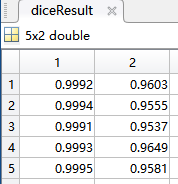

5.2 计算该组测试集的平均背景dice分割分数

讯享网%计算该组测试集的平均背景dice分割分数 meanDiceBackground = mean(diceResult(:,1)); disp(['Average Dice score of background across ',num2str(j), ... ' test volumes = ',num2str(meanDiceBackground)])

5.3 计算该组测试集的平均肿瘤前景dice分割分数

%计算该组测试集的平均肿瘤前景dice分割分数 meanDiceTumor = mean(diceResult(:,2)); disp(['Average Dice score of tumor across ',num2str(j), ... ' test volumes = ',num2str(meanDiceTumor)])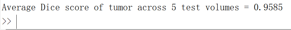

5.4 下图显示了一个箱线图(统计和机器学习工具箱)，它可视化了五个样本测试卷集合dice得分的统计数据。图中的红线显示了dice中值。蓝色方框的上限和下限分别表示dice值的第25个和第75个百分点。如果您有统计和机器学习工具箱，那么您可以使用箱线图功能来可视化所有测试集中dice分数的统计数据。要创建boxplot，请将下面代码中的createBoxplot变量设置为true。

技术问题欢迎评论留言，或者联系扣扣,共同探讨，共同进步！！！

讯享网%%创建箱线图 createBoxplot = true;%true则为创建，false则不创建箱线图 if createBoxplot figure boxplot(diceResult) title('Test Set Dice Accuracy') xticklabels(classNames) ylabel('Dice Coefficient') end

参考网站

References   ​​​​​​​

[1] Çiçek, Ö., A. Abdulkadir, S. S. Lienkamp, T. Brox, and O. Ronneberger. "3D U-Net: Learning Dense Volumetric Segmentation from Sparse Annotation." In Proceedings of the International Conference on Medical Image Computing and Computer-Assisted Intervention - MICCAI 2016. Athens, Greece, Oct. 2016, pp. 424-432.

[2] Isensee, F., P. Kickingereder, W. Wick, M. Bendszus, and K. H. Maier-Hein. "Brain Tumor Segmentation and Radiomics Survival Prediction: Contribution to the BRATS 2017 Challenge." In Proceedings of BrainLes: International MICCAI Brainlesion Workshop. Quebec City, Canada, Sept. 2017, pp. 287-297.

[3] "Brain Tumours". Medical Segmentation Decathlon. http://medicaldecathlon.com/

The BraTS dataset is provided by Medical Segmentation Decathlon under the CC-BY-SA 4.0 license. All warranties and representations are disclaimed; see the license for details. MathWorks® has modified the data set linked in the Download Pretrained Network and Sample Test Set section of this example. The modified sample dataset has been cropped to a region containing primarily the brain and tumor and each channel has been normalized independently by subtracting the mean and dividing by the standard deviation of the cropped brain region.

[4] Sudre, C. H., W. Li, T. Vercauteren, S. Ourselin, and M. J. Cardoso. "Generalised Dice Overlap as a Deep Learning Loss Function for Highly Unbalanced Segmentations." Deep Learning in Medical Image Analysis and Multimodal Learning for Clinical Decision Support: Third International Workshop. Quebec City, Canada, Sept. 2017, pp. 240-248.

[5] Ronneberger, O., P. Fischer, and T. Brox. "U-Net:Convolutional Networks for Biomedical Image Segmentation." In Proceedings of the International Conference on Medical Image Computing and Computer-Assisted Intervention - MICCAI 2015. Munich, Germany, Oct. 2015, pp. 234-241. Available at arXiv:1505.04597.

See Also

imageDatastore | randomPatchExtractionDatastore | transform | dicePixelClassificationLayer (Computer Vision Toolbox) | pixelLabelDatastore (Computer Vision Toolbox) | semanticseg (Computer Vision Toolbox) | trainingOptions (Deep Learning Toolbox) | trainNetwork (Deep Learning Toolbox)

Related Topics

• Preprocess Volumes for Deep Learning (Deep Learning Toolbox)
• Datastores for Deep Learning (Deep Learning Toolbox)
• List of Deep Learning Layers (Deep Learning Toolbox)

External Websites

• 3-D Brain Tumor Segmentation Using Deep Learning Video Tutorial