群落排序RDA验证

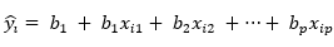
典范分析结合了排序和回归的思想，其包含一个响应变量矩阵Y和解释变量矩阵X，是与多元回归密切相关的：

讯享网
多元回归模型预测$\widehat{Y_i}$与Y的排序是不同的，二者相关系数的平方根就是多元回归模型的决定系数。因此，多元回归模型建立了$\widehat{Y_i}$排序与Y排序之间的对应，因为回归拟合值排序受限于X，并且与X是最优的且线性相关的。这个特性在典范分析中也很重要。这种限制是在最小均方（least-square）意义上最优的，意味着多元线性回归模型得到了最大的$R^2$（决定系数）。因此，典范分析结合了排序和回归的方法，在X的约束下，形成与X密切相关的Y排序。

vagan包进行RDA分析

library(vegan) library(magrittr) 

讯享网 Loading required package: permute Loading required package: lattice This is vegan 2.5-6 

spe <- read.csv("2020otuabund.csv",header=T,row.names = 1) %$% .[,-10] spe <- t(spe)[,1:16] env <- read.csv("waterc.csv",header=T,row.names = NULL) %$% .[,-(1:2)] sp <- scale(spe, center = TRUE) water <- scale(env, center = TRUE) water <- water[,c(1,2,7,8)] mod11<-rda(sp ~ TotalC+TotalN+SAL+pH, env) summary(mod11) 

讯享网 Call: rda(formula = sp ~ TotalC + TotalN + SAL + pH, data = env) Partitioning of variance: Inertia Proportion Total 16.000 1.0000 Constrained 9.832 0.6145 Unconstrained 6.168 0.3855 Eigenvalues, and their contribution to the variance Importance of components: RDA1 RDA2 RDA3 RDA4 PC1 PC2 PC3 Eigenvalue 6.5226 2.1684 0.78380 0.35745 2.7334 1.7448 1.07726 Proportion Explained 0.4077 0.1355 0.04899 0.02234 0.1708 0.1091 0.06733 Cumulative Proportion 0.4077 0.5432 0.59218 0.61452 0.7854 0.8944 0.96173 PC4 Eigenvalue 0.61228 Proportion Explained 0.03827 Cumulative Proportion 1.00000 Accumulated constrained eigenvalues Importance of components: RDA1 RDA2 RDA3 RDA4 Eigenvalue 6.5226 2.1684 0.78380 0.35745 Proportion Explained 0.6634 0.2205 0.07972 0.03635 Cumulative Proportion 0.6634 0.8839 0.96365 1.00000 Scaling 2 for species and site scores * Species are scaled proportional to eigenvalues * Sites are unscaled: weighted dispersion equal on all dimensions * General scaling constant of scores: 3. Species scores RDA1 RDA2 RDA3 RDA4 PC1 PC2 OTU72 -0.15864 -0.26192 0. -0.04309 -0. -0.02104 OTU401 -0.15190 0.41764 -0.070863 0.11729 0. 0.32065 OTU822 0.41641 -0.27951 0.074570 -0.18489 -0.0078372 0.55600 OTU334 -0.67922 0.07835 0.088613 0.04723 0. 0.20553 OTU815 0.60617 -0.41794 0. 0.09392 -0.0 0.05853 OTU828 0.64631 -0.10303 0. -0.02145 0. -0.29497 OTU461 -0.68355 -0.32370 0. 0.06208 -0.0008486 0.15978 OTU361 -0.70671 -0.23541 -0.055085 -0.03725 0.0061413 -0.04282 OTU912 0.24139 -0.18079 -0. -0.27749 -0. 0.40881 OTU83 0.46548 0.35236 0. 0.20873 -0. -0.44886 OTU638 0.52096 -0.43189 -0. 0.17608 0. -0.10085 OTU75 -0.78599 -0.08045 0.023342 -0.03683 -0.0086104 0.02925 OTU643 0.70966 0.14607 0. -0.07273 0. -0.36211 OTU868 0.59002 0.13248 0.001474 0.01602 -0. -0.33728 OTU673 0.09015 -0.67743 -0.090516 0.14908 0. -0.06191 OTU651 0.39161 0.11345 0.011508 -0.07418 0. -0.18163 Site scores (weighted sums of species scores) RDA1 RDA2 RDA3 RDA4 PC1 PC2 H1 -1.5505 -0.004236 -1.50882 -1.6763 -0.39559 -0.61280 H2 -1.6591 1. -0.59495 0.7410 0.62023 1.45094 H3 -1.4895 -2. 1.21685 0.9664 0.35000 0.01861 M1 0.2531 -0. -0.35016 -1.7639 -0.20189 0.60985 M2 0.7313 1.079749 2.39744 -0.2944 -2.09920 -0.98534 M3 0.3798 0. 0.95080 1.3976 -0.06154 -1.47745 N1 1.2253 -0. -1.90587 1.5087 -0.37623 0.01875 N2 1.2686 0. -0.28386 2.5384 2.44508 -1.06512 N3 0.8410 -0. 0.07857 -3.4175 -0.28087 2.04257 Site constraints (linear combinations of constraining variables) RDA1 RDA2 RDA3 RDA4 PC1 PC2 H1 -1.5880 0.3692 -1. -1.2108 -0.39559 -0.61280 H2 -1.3262 1.7883 -0.071104 1.1527 0.62023 1.45094 H3 -1.4864 -2.2507 1. 0.8040 0.35000 0.01861 M1 0.4777 -0.9880 -0. -1.8351 -0.20189 0.60985 M2 0.6579 0.8215 1. 0.4964 -2.09920 -0.98534 M3 -0.2408 0.5166 0.006138 -0.3785 -0.06154 -1.47745 N1 1.2080 -0.8749 -2.035604 1.8738 -0.37623 0.01875 N2 1.2022 0.4497 0. -0.1378 2.44508 -1.06512 N3 1.0956 0.1684 0. -0.7648 -0.28087 2.04257 Biplot scores for constraining variables RDA1 RDA2 RDA3 RDA4 PC1 PC2 TotalC -0.8196 -0.40984 0.33625 0.21740 0 0 TotalN -0.3354 0.35041 0.05323 0.87287 0 0 SAL -0.7938 -0.38601 -0.44072 0.16332 0 0 pH 0.9945 -0.07912 -0.02377 -0.06469 0 0 

原理验证

#计算拟合值排序矩阵、响应变量排序矩阵 XtX = t(water) %*% water invers = solve(XtX) fitY <- water %*% invers %*% t(water) %*% sp resY <- sp - fitY U <- eigen(cov(fitY))$vectors Ures <- eigen(cov(resY))$vectors FY <- sp %*% U ZY <- fitY %*% U NYres <- resY %*% Ures B = invers %*% t(water) %*% sp C = B %*% U 

讯享网var <- eigen(cov(fitY))$values #各个典范轴方差贡献 var 

 [1] 6.e+00 2.e+00 7.e-01 3.e-01 2.e-16 [6] 1.e-16 1.e-16 1.e-16 6.e-17 3.e-17 [11] 9.e-18 -1.e-17 -2.e-17 -6.e-17 -1.e-16 [16] -2.e-16 

讯享网varres <- eigen(cov(resY))$values varres 

 [1] 2.e+00 1.e+00 1.077257e+00 6.e-01 4.e-16 [6] 1.e-17 -9.e-18 -1.e-17 -1.e-17 -3.053562e-17 [11] -4.060141e-17 -4.e-17 -4.e-17 -6.e-17 -7.034357e-17 [16] -1.e-16