
In Death and Life of Great American Cities, the great Jane Jacobs lays out four essential characteristics of a great neighborhood:
在《美国大城市的死亡与生活》中 ,伟大的简·雅各布斯阐述了一个大社区的四个基本特征:
- Density 密度
- A mix of uses 多种用途
- A mix of building ages, types and conditions 混合建筑年龄,类型和条件
- A street network of short, connected blocks 短而相连的街区的街道网络
Of course, she goes into much greater detail on all of these, but I’m not going to get into all the eyes-on-the-street level stuff. Instead, I’m going to find neighborhoods with the right “bones” to build great urbanism onto. The caveat to this, as with most geospatial planning tools, is that it is not to be blindly trusted. There are a lot of details that need on the ground attention.
当然,她会在所有这些方面进行更详细的介绍,但我不会涉及所有在街头关注的内容。 取而代之的是,我将寻找具有正确“骨骼”的街区,以在其上建立伟大的城市主义。 与大多数地理空间规划工具一样,对此的警告是,不要盲目地信任它。 有很多需要地面关注的细节。
On to the data.
关于数据。
工具类 (Tools)
For this project, I’m going to use the following import statement:
对于此项目,我将使用以下import语句:
To start a session with the Census API, you need to give it a key (get one here). I’m also going to start up my OSM tools, define a couple projections, and create some dictionaries for the locations I’m interested in, for convenience:

要开始使用Census API进行会话,您需要为其提供一个密钥( 在此处获取一个)。 为了方便起见,我还将启动OSM工具,定义几个投影,并为我感兴趣的位置创建一些字典:
census_api_key='50eb4e527e6c123fcb3b526e1055ee8da' nominatim=Nominatim() overpass=Overpass() c=Census(census_api_key) wgs='EPSG:4326' merc='EPSG:3857' ada={'state':'ID','county':'001','name':'Ada County, ID'} king={'state':'WA','county':'033','name':'King County, WA'}讯享网
These two are interesting because they have both seen significant post-war growth and have a broad spectrum of development patterns. As a former Boise resident, I know Ada County well, and can provide on-the-ground insights. King County has a robust data platform that will allow for a different set of insights in part II of this analysis.
这两个很有趣,因为它们都在战后取得了长足的发展,并拥有广泛的发展模式。 作为博伊西省的前居民,我非常了解Ada县,并且可以提供实地见解。 金县拥有强大的数据平台,该平台将在本分析的第二部分中提供不同的见解。
密度 (Density)
We’ll start off easy. The U.S. Census Bureau publishes population estimates regularly, so we just need to put those to some geometry and see how many people live in different areas. The smallest geography available for all the data that I’m going to use is the tract, so that’s what we’ll get.
我们将从简单开始。 美国人口普查局会定期发布人口估算值,因此我们只需要将其估算为某种几何形状,并查看有多少人居住在不同地区。 对于我将要使用的所有数据,可用的最小地理区域是区域,这就是我们要得到的。
讯享网def get_county_tracts(state, county_code): state_shapefile=gpd.read_file(states.lookup(state).shapefile_urls('tract')) county_shapefile=state_shapefile.loc[state_shapefile['COUNTYFP10']==county_code] return county_shapefile
Now that I have the geography, I just need to get the population to calculate the density. The Census table for that is ‘B01003_001E,’ obviously. Here’s the function for querying that table by county:
现在我有了地理,我只需要获取人口来计算密度。 显然,人口普查表是“ B01003_001E”。 这是按县查询该表的函数:
def get_tract_population(state, county_code): population=pd.DataFrame(c.acs5.state_county_tract( 'B01003_001E', states.lookup(state).fips,'{}'.format(county_code),Census.ALL)) population.rename(columns={'B01003_001E':'Total Population'}, inplace=True) population=population.loc[population['Total Population']!=0] return populationNow that we have a dataframe with population, and a geodataframe with tracts, we just need to merge them together:
现在,我们有了一个包含人口的数据框和一个具有区域的地理数据框,我们只需要将它们合并在一起:
讯享网def geometrize_census_table_tracts(state,county_code,table,densityColumn=None,left_on='TRACTCE10',right_on='tract'): tracts=get_county_tracts(state, county_code) geometrized_tracts=tracts.merge(table,left_on=left_on,right_on=right_on) if densityColumn: geometrized_tracts['Density']=geometrized_tracts[densityColumn]/(geometrized_tracts['ALAND10']/.1103) return geometrized_tracts
This function is a little more generalized so that we can add geometries to other data besides population, as we’ll see later.
对该函数进行了更概括的描述,以便我们可以将几何体添加到人口总数以外的其他数据中,我们将在后面看到。
Now we can simply call our function and plot the results:
现在,我们可以简单地调用函数并绘制结果:
ada_pop_tracts=geometrize_census_table_tracts(ada['state'],ada['county'],get_tract_population(ada['state'],ada['county']),'Total Population') ada_density_plot=ada_pop_tracts.plot(column='Density',legend=True,figsize=(17,11))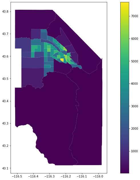
版权声明:本文内容由互联网用户自发贡献,该文观点仅代表作者本人。本站仅提供信息存储空间服务,不拥有所有权,不承担相关法律责任。如发现本站有涉嫌侵权/违法违规的内容,请联系我们,一经查实,本站将立刻删除。
如需转载请保留出处:https://51itzy.com/kjqy/115572.html